Clustering algorithm to approximate functions

In the last post we discussed about function approximation through polynomials having exponents in the Real domain.
We have also seen that to obtain a good approximation of the function, long training session is required; the reason of this inefficiency lays in one and on the gradient surface and in another hand on the strategy adopted to train the system.
Let me spend few words about the gradient surface:

The gradient surface conformation is strictly related with the number of monomials used to approximate functions, so

• if you use fews monomials the approximation cannot be good because you are using less complexity respect the complexity of the original function and the gradient will have pretty regular convex surface with bottom equal to best approximation achievable by the linear combination of monomials chosen.
• if you use too many monomials, you are building a complex gradient function (because the number of its parameters are growing), so you increase the risk to fall down in a local minimum.

I mentioned that annealing strategy can help to overcome the barriers imposed by local minimums, but for the time being I prefer show you a little bit more sophisticated strategy: the clustering learning.
As you know usually the clustering techniques are used to divide data in different categories, but I would like once again deliver the message that in data mining (and in text mining as well) what is real important is not the product, the tool or the suite, but the knowledge, the creativity and the skills to abstract the problems and the algorithms and adapt the second one to solve the first one.

Divide et Impera (Latin motto)
... that is divide the problem in sub problems, find sub solutions and merge them to obtain the overall solution.
The strategy is very easy to describe:
1. Divide the domain of your function in k sub intervals.
2. Initialize k monomials;
3. Consider the monomials as centroids of your clustering algorithm.
4. Assign the points of the function to each monomial in compliance to the cluster algo.
5. Use the gradient descent to adjust the parameters of each monomial.
6. Go to 4. until the accuracy is good enough.

Basically in the former version we had this approximation:

Function Approximation through power real polynomials

While in this approach we introduce the membership of function which assign each point to each cluster (in this case monomial)

Power Real Polynomials approximation with clustering approach

Let's see the result obtained with the sinusoid function (please compare with the former results obtained with the canonical gradient descent).

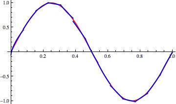
Clustering approach to fit the Sin(x) function

Let me show how these strategy works in more complex domains, for example in R^3 (of course you should add extra "y" variable to the monomial).
First Example

And here you are the monomials found and the fitting found applying the membership function (I choose a crispy version but it is also feasible a fuzzy approach):

The spheres represent the points belonging to the original function, while the planes are representing the monomials surface found by clustering & gradient. (approximation with 36 monomials)

And the fitting obtained:

Original Function depicted with  blue points; Fitting depicted with Orange Points  

Second Example
The function chosen is the following:

On the left side the original function,
 on the right side the hyperplanes (monomials) found by gradient descent cluster based.

The fitting obtained applying the above monomials and the membership function:

The graphs shows the plane described by the original function.
In blue the  points belonging to the original function.
In orange the fitting obtained using the clustering based procedure.

As usual: Stay Tuned 

Cristian

Power Real Polynomial to approximate functions: The Gradient Method

In the real world rarely a problem can be solved using just a single algorithm, more often a solution is a chain of algorithms where the output of the former is the input for the follower.

But you know that quite often machine learning algorithms return functions almost always extremely complex, and they don’t fit directly in the next step of your strategy.

In these conditions, it is really helpful the trick of the function approximation, that is, we reduce the complexity of our original model using a new easier model.

The big advantage of the function approximation is that you can impose the form of new model to describe your data.

One of the most common “model” used is the polynomial approximation (also know with the term linearization).

As you can imagine the polynomial approximation takes vantage of the linear combination of monomial and it makes easier analytical approaches.

First approach: Polynomial fitting (power-real) gradient descent

To apply this approach your simplified model must be differentiable!

I don’t want spend time explaining how to implement it because it is so standard and common that it is available everywhere on internet.

In my toolbox there is always a notebook with the gradient descent implementation: it is so general purpose that I couldn’t leave without it!!

Let me show a quick demonstration of it on two different cases:

In the first one I found an approximation of Sin[x] (…In a real scenario I would be really happy to have a “complex” model following a Sin function).

Polynomial approximation for Sin(x): A good approximation obtained after 30.000 iterations.
(In red the original function, in orange the approximation)

In the following case I choose a much complex function: 

And the results for this example is:

Polynomial approximation: here the convergence required six monomials and 70.000 iterations.
The final results has obtained via "fine-tuning" and it took 5000 iterations.
(In red the original function, in orange the approximation)

In both example the convergence has been measured like the square error respect the target function.

Considerations:

• If you increase the number of the monomials, you are increasing the risk to fall in a local minimum.
•  You should start with very small values of eta learning (I usually use two different eta learning: the first one for the coefficients and the second one for the exponents).
• To speed up the convergence you should increase incrementally the value of eta learning.
• To refine the learning it could be useful  "Fine tuning"  presenting samples with asymmetric distribution to focus the learning on the tricky regions.

Of course this strategy requires a bit of experience to be used and good dose of patient!

Be aware that the approximation as just local effects: if you move far away the training region, the error increase dramatically.

In the next session I show how to increase the accuracy of this technique mixing the gradient descent with simulated annealing.

Stay tuned.