Support Vector Clustering: An approach to overcome the limits of K-means

Time ago, I posted a banal case to show the limits of K-mean clustering. A follower gave us a grid of different clustering techniques (calling internal routines of Mathematica) to solve the case discussed.
As you know, I like write by myself the algorithms and I like show alternative paths, so I've decided to explain a powerful clustering algorithm based on the SVM.
To understand the theory behind of SVC (support vector clustering) I strongly recommend  to have a look at: http://jmlr.csail.mit.edu/papers/volume2/horn01a/rev1/horn01ar1.pdf . In this paper you will find all technical details explained with extremely clearness.
As usual I leave the theory to the books and I jump into the pragmatism of the real world.
Consider the problem of a set of points having an ellipsoid distribution: we have seen in the past that K-means doesn't work in this scenario, and even trying different tweaks changing the position of the centroids and its number of centroids, the final result is always unacceptable.
SVC is a clustering algorithm that takes in input just two parameters (C and q) both of them real numbers. C is to manage the outliers and q is to manage the number of clusters. Be aware that q is not directly related with the number of clusters!! Tuning q  you can manage the "cluster granularity" but you cannot decide a priori the number of clusters returned by the algo.


How to implement SVC.
There are many implementations of SVC, but I would like to show different tools (I love broaden the horizons...), so the ingredients of the daily recipe are: AMPL & SNOPT.
Both of them are commercial tools but to play with small set of points (no more than 300) you can use for free the student license!
AMPL is a comprehensive and powerful algebraic modeling language for linear and nonlinear optimization problems, in discrete or continuous variables and SNOPT is a software package for solving large-scale optimization problems (linear and nonlinear programs).
AMPL allows the user to write the convex problem associated to SVC's problem in easy way:

The AMPL file for SVC

And SNOPT is one of the many solvers ables to work with AMPL.

In the former image, after the statement "param x: 1  2   3   :=" there are the list of 3D points belonging to our data set.

One of the characteristics of SVC is the vector notation: it allows to work with high dimensions without changes in the development of the algorithm.

2D Problem 
Let's show the application of SVC in our ellipsoid data set

300 pt having ellipsoid distribution.  The first contour of SVC  has been depicted in black.   

The above image shows the clusters (depicted like connected components of a graph...read further details in the mentioned paper) returned by SVC and plotted by Mathematica.

3D problem
Just to show the same algorithm working in 3D on the same problem:

3D points having ellipsoid distribution.

And Here you are the SVC results plotted by Mathematica:

SVC applied on the former data set

As you can see in both scenarios SVC is able to solve the easy  problem that K means cannot manage.

PS

We will continue the text categorization in the next post... From time to time I allow to myself some divagation. 

How the classifier accuracy is conditioned by the Feature Set (Bag of words)

In the last post we have seen a naïve approach to classify via SVM and C5, and we noticed that both SVM and C5 didn’t get good accuracy.

Despite the unsatisfactory results, we tested the different algorithms under the same conditions, and we found out that (at least in this case) they have the same behavior. Of course we should repeat the test in different conditions to provide a correct benchmark: in a next time we will do that.

But right now, I would like to perform a more useful (for our classification target) benchmark-test:

Consider an SVM based classifier, trained using the same parameters tuning strategy: How does the accuracy change if we build the vectors using different bag of words?

Basically we are trying to understand what is the best strategy to select the feature set (that is the bag of words) to classify our 4–classes data set.

Let me clarify immediately an important point:

• The strategy of “single bag of words” isn’t an approach really useful in real business scenarios: it is too much trivial.

So why are we doing such test?

Because these kind of tests can give us a lot of useful information about the data set, and allow us to choose the best strategy!

Test description.

We have already seen that measure the accuracy on the training set is extremely dangerous (soon or later I should explain the pillar of error theory and the overfitting problems…).

So the first step is to assess your experiment with a validation set (...there are more sophisticated test to do that like k-fold cross validation, but for our case should be enough): How can we do that?

…Easy: splitting the training set in two parts: the first one will be used to train the algorithm, and the second one will be used to measure the accuracy.

Be aware: you never can measure the accuracy using samples already observed by the learning algo. Of course you cannot measure the accuracy on the test set to retraining your system!! (please see the article of dr. Sandro Saitta at: http://www.dataminingblog.com/how-to-cheat-with-data-mining).

Training Set splitting

The second step is to build the vectors of the same training set using different bag of words. For this experiment, I used the “TF-DF”, “TF-IDF”, and the “Closeness Centrality” functions to extract the features and to build the vectors.

At this point we can assess the accuracy of the classifier with the same data set but built in different ways.

Accuracy test using TF-DF bag of words.
In the accuracy matrix (% format) the principal diagonal contains the true positive.  

Accuracy test using TF-IDF bag of words.
In the accuracy matrix (% format) the principal diagonal contains the true positive.

Accuracy test using Closeness Centrality based bag of words.
In the accuracy matrix (% format) the principal diagonal contains the true positive.  

The above tables shows (in percentage) the answers provided by the classifier (the diagonal are the True Positive). The element [i,j] = x says that: the real class was i and the classifier assigned to the class j x% of the documents belonging to i.

For the "graph theory based" bag of words, we can also shown the corpus distribution in terms of the closeness function:

Graph of the Corpus generated by Closeness Centrality (has been plotted only the most relevant features)
Red color = high Closeness Centrality.
Purple = low Closeness Centrality.  

Results

There are three important things to highlight:

1. For this data set the TF-DF feature set returns the worst accuracy (the grain class TP = 43%) respect the other two methods.
2.  The TF – IDF and the Closeness Centrality give better results. And the accuracy is almost identical in absolute terms.
3.  The grain and oil classes are the tricky case: the algorithm is not able to divided them properly.

As you can imagine the third findings is the most important information returned by this experiment: it says us that we have to spend more efforts to highlight the differences among the classes oil and grain in order to increase the accuracy.

Notice that in the “TF - IDF” and “Closeness Centrality” the True Positive distribution is mirrored! This supports our thesis that we are not describing properly the documents belonging to these two classes.

We will see how to solve the problem!

Stay Tuned.

Classification Step: C 5.0 vs SVM

Finally, after many preambles we have all conditions to classify the documents. So far we have seen:

1. How to translate a document in a vectors understandable by algorithms;
2. How to analyze the data set with density analysis;
3.  How to reduce the dimension of the problem (features reduction)

Well, now we have the all ingredients to classify the documents.

To show a couple of approach, I have extracted 4 classes from our REUTERS data set (choosing the criteria “TOPICS”, and considering the easier condition of documents belonging only to one class): “GOLD”,“GRAIN”,”OIL”,”TRADE”.

In this stage I put my self in a “comfortable zone” so, I considered the easiest way to classify the documents, that is, I built the vectors considering just ONE “bag of words”.

Basically I extracted the features set from the entire training set without any distinction of the specific class of the document.

In this approach we are delegating the entire complexity of the task to the classifier!

As we can see below, be lazy never pay!! (…I hope that it makes sense in English… ).

Let’s move on the results.

As I always recommend, never play with one toy! Be always curios and try different approach to solve the problem.

In this spirit for the time being I have done some tests using SVM (in LIBSVM implementation) and C.5 (the free version).

I embedded in Wolfram Mathematica the scripts to run both LIBSVM and C5 (contact me at cristian.mesiano@gmail.com if you desire the source); in this way all tasks (data preparing, features extraction, vector building and so on) can be done using only one interface.

Here you are the accuracy for SVM: 

Notice that the training set has been rescaled and weighted with different scores. 

Accuracy For SVM Classifier: Best results with Linear Kernel

As you can see, the accuracy measured on the training set is not brilliant! The OIL class is in the 50% of the case mislead. Moreover we have to consider that:

·      we are working with an easy data set and with few classes.

·      The accuracy has been measured only on the training set (…remember that the first error of the newbie is to focus much more on the training env.). The training set contains only points already observed by the classifier.  And analysis done only on it can hide overfitting problems!!

Even trying with different tuning, and with different kernels, the accuracy doesn’t improve.

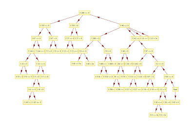
The situation doesn’t improve with C5: as you can see below, the accuracy is pretty much the same achieved via SVM.

The Decision Tree returned by C5 (plotted with Mathematica). 

Accuracy Matrix Provided by C5: The results are pretty similar to the SVM computations 

So Do we give up?

NEVER.

In the next posts we will see how improve the accuracy introducing boosting techniques.

…There are thousands of details to consider and to explain like:

linear kernels for SVM, how to measure the accuracy, how to improve the training set and avoid the over fitting…

We will see that in the next posts.

Stay Tuned

Cristian