Function minimization: Simulated Annealing led by variance criteria vs Nelder Mead

Most of the datamining problems can be reduced as a minimization/maximization problem.
Whenever you are looking for the best trade off between costs and benefits you are solving a minimization problem.

Often the number of the variables that affects the cost function is high and the domain of these variables is in a dense set and, last but not least: in the real world problem often, you have no clue about the analytical form of the function.
Formally such problems belong to the multidimensional unconstrained optimization family.

Examples

Let's consider  easy scenarios where the function cost is conditionated just by two parameters.

Schaffer f6 function: in the contour plot  dark purple to depict local minimums.

Another function where minimum ischaracterized by two valleys 

This function presents several local minimums well depicted in the contour plot

This function is characterized by a several local minimums having high range of values 

As you can see the above problems have in common a massive presence of local minimum :).

Let's see how to handle these problems through an approach that I define hybrid, that is, obtained mixing different methods and properties.

Simulated Annealing (SA) "variance based" approach

Disclaimer: I had no the time to check whether this method has been already published somewhere. The underlying idea is quite simple, so I would assume that someone has already spent time in proofing convergence and better variations (and actually I don't think is a rocket science proof it).

SA, belongs to the family of numerical method based on "search strategy" and its convergence requirements are related to the stationary conditions inducted by the underlying markovian process.

In a former post I showed an its application in a discrete domain, where at each iteration we chose the next candidate solution by comparison with the current solution. The new solution was found "fishing randomly" a candidate in a discrete space.

In the above problems the solution space is continuos, so we need a smart strategy to extract the new candidate. Let's see my approach!

Variance trick 

Let's consider a sampling in two different region of a function f :

• sampling_1 in a region having a smooth minimum and evaluate such points
• sampling_2 in a region having a spiky minimum and evaluate such points

Take now the variance of these evaluated sets.
How does the variance of f(sampling_1)  change respect the variance of f(sampling_2)?  
Here you are the answer:

As you can see the variance can be used as indicator of a minimum region of the cost function.

Instead of explore randomly the solution space, the approach I propose is led by the variance used as  above. 

What happens if the smooth valley is a global minimum?

There are two intuitive factors to avoid that the algorithm jams in a local minimum:

1. The acceptance law admit also pejorative solutions.

2. The sampling procedure moderate by variance (if the variance is chosen high enough) allows explorations of better regions.

The algorithm

The meta code of the Simulated Annealing based on variance criteria

Many optimizations can be done to the algorithm.

For instance we could condition the annealing procedure only if the

argMin(evaluate(f,newSet)) > argMin(evaluate(f,curset))

Tests
Let's see how the approach works.
As usual, all my experiments are compared with other techniques. In this case I chose as comparative method the well known "Nelder Mead" method.
I tried to optimize the Nelder Mead method playing around its param setting: shrink ratio, contraction ratio and reflection ratio.
All experiments have been done using the same initial points.
For the Nelder Mead method I plotted just the unique solutions found.
The approach I propose has been led using always the same setting (3000 cycles, variance sampling = 0.75).
Experiment 1.

On the left side it has been represented the solution found by Nelder Mead method.
On the right side the solution found by the SA presented in this post: the blue point depicts the starting point and the red point depicts the solution found.
The last chart shows the space solution explored.

Notice that method found a better solution respect Nelder Mead approach. 

Experiment 2

On the left side it has been represented the solution found by Nelder Mead method.
On the right side the solution found by the SA presented in this post: the blue point depicts the starting point and the red point depicts the solution found.

SA found a better solution in really few steps.

Experiment 3

On the left side it has been represented the solution found by Nelder Mead method.
On the right side the solution found by the SA presented in this post: the blue point depicts the starting point and the red point depicts the solution found.

This experiment shows once again the good performance of this approach even if the problem is very challenging!

Experiment 4

On the left side it has been represented the solution found by Nelder Mead method.
On the right side the solution found by the SA presented in this post: the blue point depicts the starting point and the red point depicts the solution found.

The convergence, as shown above, has been reached very quickly.

Conclusion

The approach seems promising and works well in different contexts:  I'm quite sure that many improvements can be implemented.

I'm looking forward to receive your comments, ideas and other comparative tests.

Stay tuned!

cristian

Data Mining: Tools and Certificates

As member of many Linkedin groups related to data mining & text mining I read many threads related to certificates that should help either in job seeking and consolidating curriculum, and many other threads about miraculous tools able to solve whatever problem.
Is being certified really worth it?
In my experience I think that a certificate in a specific data mining tool could be a positive point on the curriculum, but it doesn't really help to improve your knowledge on the field.
Let me explain better (which is not easy with my bad English): The certificates system is a market and its target is to generate profit or to promote products.

Data mining tools
My question is: do you really think that can exist a tool able to embrace all aspects related to data mining?

I guess that the number of problems data mining related are so high that maybe we could use the Cantor diagunalization to proof that are uncountable :)

In my opinion is too naive the common thought that through a software, clicking here and there you can obtain tangible benefits in mining your data.
The "data mining" definition has been created by marketing industries just to summarize in a buzz word  technics of applied statistics and applied mathematics to the data stored in your hard disk.
I don't want say that tools are useless, but it should be clear that tools are only a mean to solve a problem, not the solution.

• In the real world the problems are never standard and really seldom you can take an algorithm as is to solve them! ...maybe I'm unlucky but I never solved a real problem through a standard method.
• The tool X is able to load Terabyte of data. And so what? A good data miner should know that you cannot consider the entire population to analyze a phenomena, you should be able to sample your population in order to ensure the required margin of accuracy! ... this technic is simply called Statistic!
• If you really want to claim "I know very well this approach", you must be able to implement it by your self: only implementing it by your self you can deeply understand in which context the algorithm works, under which conditions it performs better than other tools and so on. Don't rely only on one paper that compare few techniques: if you change just one of the conditions the results are terrible different.
• Without theory you cannot go deep: Let's consider a tool as Mathematica or R or ... These tools allow the user to have access to a large library of pre defined algorithms and routine, they provide visualization functions to show results in a fancy way, and last but not least they provide a complete language programming to code whatever you want. I love them, but I couldn't do anything without the theory behind the problem. Mathematica can provide me the algorithm to cluster a data set through k-means: but how can I be sure that it is the right algo for your problem? (click here to have a demo).

Actually I would prefer attend a course to deepen some aspects of multivariate statistic or seminars on new methodology to solve some problem respect pay plenty money to know every single detail of a tool, that maybe will not be in the market in the next 5 years.

I know that the companies often are looking for certified guys on a famous tool just because they bought it and they need to reduce the time to "integrate" a new resource on a team. Fair enough! ...but I think it is ridiculous require certificates as strict requirement!

I'm really curious to know your experiences and opinions.
cristian

Simulated Annealing: How to boost performance through Matrix Cost rescaling

One of the most widely algorithm used in Machine Learning is the Simulated Annealing (SA).
The reason of its celebrity lays in:

• Simplicity of implementation
• broad spectrum of applicability

There are many implementations of it available for almost all languages, and many books and papers on the topic; personally the best book I would like to suggest is the Simulated Annealing and Boltzmann Machines: A Stochastic Approach to Combinatorial Optimization and Neural Computing wrote by Korst & Aarts.

The problem
In this post I'm going to describe a very canonic combinatoric problem (NP hard complexity) often approached through annealing methods: the complete Asymmetric Travelling Salesman Problem (ATSP).
The ATSP problem, as you know, can be taken as base to model several problems as for instance network routing problems, chemistry and physics problems. The ATSP is so charming (at least for me) because the nature of the problem is very easy and the way to find out the best solution is extremely trivial: you have to explore all the possible solutions!
The only problem is the number of solutions you have to compare:

• with 10 towns you have to explore ~ 3.6*10^6 solution.
• with 50 towns you have to explore ~ 3 *10^64 solution.

In the past (I'm not aware if it is still open) there were many competitions to find the best solution of the asymmetric and complete TSP with more than 30000 towns.

...Considering the time required to obtain the optimal solution, in many cases a sub optimal solution obtained exploring less than 1% (as usually happens with SA) of the solution space could be enough!


The experiments
I considered two instances of the problem, the first one with 10 towns and the second one with 50 towns.
Even if for this kind of problem there are more efficient algorithms to face TSP, I chose the simulated annealing just to show how versatile it is and to show how much the rescaling operation is essential in order to maximize the performance of your algorithm. 

Why rescaling? (I'll try to be technical as little as possible)
The SA bases its powerful on the ability to overcome the local minimum through the acceptance at time "t" of a bad solution respect a better solution found at the time "t-1". It assigns an acceptance probability based on the sigmoidal function that decrease if the cost of the new solution is higher respect the current solution.
So if the cost distance between the current solution and the new solution is very high, the acceptance probability will be very small.
This probability is mitigated by the temperature schedule that allow more acceptance rate (of bad solutions) when the temperature of the system is high, and it is reduced once the temperature of the system decreases during the exploration of the solution space.
The aim of the rescaling is to increase the distance between towns having high cost and to reduce the cost of short distance between towns.
To obtain it I apply a "quasi" n log n function to the cost matrix.
(A publication on the topic should be ready by the end of the year).

Results
All experiments as usual as been done through "home made" application written in Mathematica.

• The cost matrix has been built  using a uniform distribution with integer values (1 to 10 for the first experiment and 1 to 100 for the second one).
• Just to have a reference point I assigned to the cost matrix the minimum value (1) in correspondence of the external perimeter of the "town system"
• The ATSP with 10 towns has optimal solution cost = 9. The ATSP with 50 towns has optimal solution cost = 49.

After 2000 cycles, SA found a solution having cost = 13. (the graph on the II quadrant represents the acceptance prob.).
The initial temperature beta has been set = 5.

After 1000 cycles, SA with MatrixCost rescaled found the optimal solution having cost 9.
The initial temperature beta has been set = 5.

I repeated the same experiment increasing the initial temperature to 15.

SA launched with beta= 15. After 5000 cycles the sub optimal solution found has cost = 14

SA with matrix cost rescaled after 2000 cycles found better solution (same initialization of the above experiment)

A larger test has been done to understand the statistical behavior:

The blue line represents the solution costs of the traditional SA.
The red line represents the solution costs of the SA with matrix cost rescaled 

And to conclude, here you are the results obtained with higher complexity (50 towns).

ATSP (50 towns) comparison between traditional SA and SA with rescaled matrix cost.

Let's try to increase the number of cycles from 1000 to 3000.

The % of success of the new strategy seems increase with the increase of the number of cycles.

Let's see what happens increasing once again the number of cycles:

The assumption seems to be confirmed: the new strategy performs better than the traditional SA even if the number of cycles is higher. 

Conclusion

1. Often the accuracy/performance of an algorithms depends on the way you feed it with the data! Rescaling your data is quite always essential!
2. The strategy requires further tests and validation.

...We will discuss about the function used to rescale the matrix costs and some other application of SA on different problems in the next posts.

cheers & stay tuned

P.S.

Special thx to Tom V. : he is on the top of the list of the contributors for the sponsorship program.

Outlier analysis: Chebyschev criteria vs approach based on Mutual Information

As often happens, I usually do many thing in the same time, so during a break while I was working for a new post on applications of mutual information in data mining, I read the interesting paper suggested by Sandro Saitta on his blog (dataminingblog)  related to the outlier detection. 

...Usually such behavior is not proficient to obtain good results, but this time I think that the change of prospective has been positive!


Chebyshev Theorem
In many real scenarios (under certain conditions) the Chebyshev Theorem provides a powerful algorithm to detect outliers.
The method is really easy to implement and it is based on the distance of Zeta-score values from k standard deviation.
...Surfing on internet you can find several explanations and theoretical explanation of this pillar of the Descriptive Statistic, so I don't want increase the Universe Entropy explaining once again something already available and better explained everywhere :)


Approach based on Mutual Information
Before to explain my approach I have to say that I have not had time to check in literature if this method has been already implemented (please drop a comment if someone find out a reference! ... I don't want take improperly credits).
The aim of the method is to remove iteratively the sorted Z-Scores till the mutual information between the Z-Scores and the candidates outlier I(Z|outlier) increases.
At each step the candidate outlier is the Z-score having the highest absolute value.

Basically, respect the Chebyschev method, there is no pre-fixed threshold.

Experiments
I compared the two methods through canonical distribution, and at a glance it seems that results are quite good.

Test on Normal Distribution

As you can see in the above experiment the Mutual information criteria seems more performant in the outlier detection.

Test on Normal Distribution having higher variance

The following experiments have been done with Gamma Distribution and Negative Exponential

Results on Gamma seem comparable.

Experiment done using Negative Exponential distribution

...In the next days I'm going to test the procedure on data having multimodal distribution.
Stay Tuned
Cristian

Uncertainty coefficients for Features Reduction - comparison with LDA technique

We have already discussed about feature selection and features reduction, and all the techniques we explored were strictly related and applicable only in the text mining domain.

I would to show you one method very powerful, easy to implement and extremely general, because it is not related to the nature of the problem.

The method is known as coefficients of constraint (Coombs, Dawes and Tversky 1970) or uncertainty coefficient (Press & Flannery 1988) and it is based on the Mutual Information concept.


Mutual Information
As you know, the Mutual Information between two random variables X and Y I(X,Y) measures the uncertainty of X knowing Y, and it says how much the uncertainty (entropy) of X is reduced by Y.
This is more clear looking at the below formula:

I(X,Y)= H(X)-H(X|Y)

Where H is the Entropy functional.

As usual, I don't want enter in theoretical discussions, but I heartily recommend a deep read of the book Elements of Information Theory: In my opinion it's the best book in that field.

Let's now rethink the mutual information as a measure of "how much helpful is the feature X to classify documents having  label L":

I(L,X) = H(L)-H(L|X)

So, for each label and each features we can calculate the features ranking!

Of course you can consider the average of I(L_i,X) for each label L_i, or also more complex function over that. BTW you have to assign higher rank to the feature Xj that maximize all I(L_i,Xj).

Uncertainty coefficient

Consider a set of people's data labelled with two different labels, let's say blue and red, and let's assume that for this people we have a bunch of variables to describe them.

Moreover, let's assume that one of the variables is the social security number (SSN) or whatever univocal ID for each person.

Let me do some considerations:

1. If I use the SSN to discriminate the people belonging to the red set from the people belonging to blue set, I can achieve 100% of accuracy because the classifier will not find any overlapping between different people.
2. Using the SSN as predictor in a new data set never seen before by the classifier, the results will be catastrophic!
3. The entropy of such variable is extremely high, because it is almost a uniform distributed variable!

The key point is: the SSN variable could have a great  I value but it is dramatically useless to classification job.

To consider this fact in the "mutual information ranking", we can divide it by the entropy of the feature.

So features as SSN will receive lower rank even if it has an high I value.

This normalization is called uncertainty coefficient.

Comparative Experiment

Do you have enough about the Theory? I know that ... I did all my best to simplify it (maybe to much...).

I did some tests on the same data set used in this paper by Berkley University:

BleiNgJordan2003.pdf.

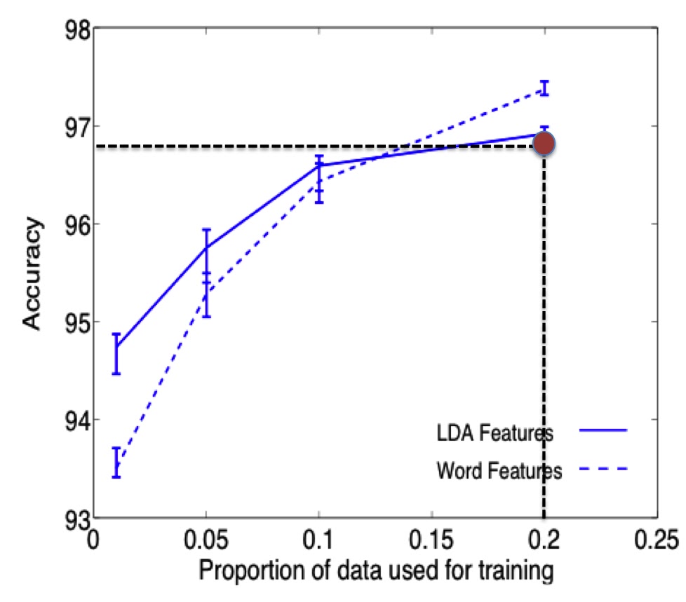
In this test the authors did a boolean experiment over REUTERS data set (actually it is very easy test) and they compared the accuracy obtained using all the words in the data set as features and the features extracted through a Latent Dirichlet Allocation method.

The data set contains 8000 docs and 15818 words. In the paper they claimed that they reduced the feature space by 99.6% and they used the entire data set to "extract" the features.

Under this condition they tested using no more than 20% of the data set as training set.

In the comparative test I focused on the second experiment mentioned: GRAIN vs NOT GRAIN.

Here you are the process I followed:

1. I choose as training set 20% of the docs.
2. from the above training set I extracted (after stemming and filtering process) all the words and I used them to build the boolean vectors.
3. I ranked the words through the uncertainty coefficient.
4. I extracted the first 60 features: that is only 0.38% of the original feature space
5. I trained an SVM with a gaussian kernel and very high value of C
6. I tested over the remaining 80% of the data set.

Before the results, let me show you some graph about the feature ranking.

Entropy of the first 3000 features.

The above graph shows the entropy of the first 3000 features sorted by TF-DF score.
As you can notice, the features having low score have low entropy: it happens because these features are present in really few documents so the distribution follows a Bernulli's distribution having "p" almost equal to 0: basically the uncertainty of the variable is very small.


Here you are the final ranking of the first 2500 features. 

Uncertainty coefficient for all features.

Results

The overall accuracy measured over the test set is equal to 96.89% and it has been depicted in the below graph (I used their original graph [figure 10.b] as base) as a red circle:

Accuracy comparison: the red circle represents the accuracy obtained training an SVM with the features extracted through the Uncertainty Coefficients.

I would like to remark that the features has been extracted using just the training set (20% of the data set),  while the experiments done by the authors of the mentioned paper used the entire data set.

Better results can be easily achieved using the conditioned entropies in an iterative algorithm where the mutual information is measured respect a local set of features (adding the features that maximize the M.I. of the current set of features).

Our  experiment shows clearly that the "Uncertainty Coefficients" criteria is a really good approach!

Soon, we will see how to use this criteria to build a clustering algorithm.  

As usual: stay tuned.

cristian

Earthquake prediction through sunspots part II: common Data mining mistakes!

While I was writing the last post I was wondering how long before my followers notice the mistakes I introduced in the experiments.
Let's start the treasure hunt!
1. Don't always trust your data: often they are not homogeneous.
In the post I put in relation the quakes in the range time between [~1800,1999] with the respective sunspots distribution.

A good data miner must always check his dataset! you should always ask to yourself whether the data have been produced in a congruent way.
Consider our example: the right question before further analysis should be: "had the quakes magnitude been measured with the same kind of technology along the time?"
I would assume that is dramatically false, but how can check if our data have been produced in a different way along the time?
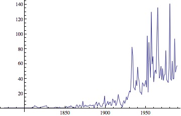
In this case I thought that in the past, the technology wasn't enough accurate to measure feeble quakes, so I gathered the quakes by year and by the smallest magnitude: as you can see, it is crystal clear that the data collected before 1965 have been registered in different way respect the next period.

The picture highlights that just major quakes (with magnitude > 6.5) have been registered before 1965.
This is the reason of the outward increasing of quakes!

... In the former post I left a clue in the caption of "quakes distribution" graph :)

In this case the best way to clean up the dataset is to filter just quakes having magnitude grater than 6.5.

Let me show you a different way to display the filtered data: "the bubble chart".

The size of the bubble is representative of the magnitude of the quakes 

The size of the bubble is representative of the number of the quakes

I love the bubble chart because it is really a nice way to plot 3D data in 2D!!

2. Sampling the data: are you sampling correctly your data?

In the former post I considered only the quakes registered in USA. 

Is it representative of the experiment we are doing?

The sunspots should have effects on the entire Earth's surface, so this phenomena should produce the same effects in every place.

...But as everybody knows: there are regions much more exposed to quakes respect other areas where the likelihood to have a quake is very low.

So the right way to put in relation the two phenomena is to consider the World distribution of the quakes.

3. Don't rely on the good results on Training Set.

This is maybe the worst joke I played in the post :) I showed you very good results obtained with the support regression model.

...Unfortunately I used the entire data set as training set, and I didn't check the model over a new data set!

This kind of mistake in the real scenario, often generates false expectation on your customer.

The trained model I proposed seemed very helpful to explain the data set, but as expected it is not able to predict well :(.

How can you avoid the overfitting problem? The solution of this problem is not so trivial, but in principle, I think that cross validations techniques are a safe way to mitigate such problem.

Here you are the new model:

The left graph shows the Training Set (in Blue the number of quakes per year, in Red the forecasting model).
The graph on the right side shows the behavior of the forecasting model over a temporal range never seen before by the system. The mean error is +/-17 quakes per year.

The Magnitude forecasting
(on the left the training set, on the right side the behavior of the forecasting model over the test set).
The mean error is around +/-1.5 degrees.

Considering the complexity of the problem I think that the regressor found works pretty good.

Just to have a better feeling of how the regressor is good, I smoothed the data through a median filter:

Moving Median Filtering applied to the Magnitude regressor.

Looking at the above graph, it seems that the regressor is able to follow the overall behavior.

As you can see such filtering returns a better understanding of the "goodness" of your models when the function is quite complex.

4. You found out a good regressor, so the phenomena has been explained: FALSE.

You could find whatever "link" between totally independent phenomena ... but this link is just a relation between input/output. nothing more, nothing less.

As you know this is not the place for theorems, but let me give you a sort of empirical rule:

"The dependency among variables is inverse proportional to the complexity of the regressor".

As usual stay tuned.

Cristian

Support Vector Regression (SVR): predict earthquakes through sunspots

In the last months we discussed a lot about text mining algorithms, I would like for a while focus on data mining aspects.
Today I would talk about one of the most intriguing topics related to data mining tasks: the regression  analysis.
As you know the regression analysis is an approach to modeling the relationship between a set of variables "y" and  explanatory variables "x" (called regressor).
The model I've chosen to talk about regression is strictly related to the SVM algorithm already presented in our classification problems: Support Vector Regression (SVR).


How does it work?
In SVR the basic idea is to map the data x into a high-dimensional feature space F via a nonlinear mapping  and to do linear regression in this space.


Why SVR?

• SVR is extremely robust even in input space having high dimension because the optimization doesn't depend on the dimension of input space.
• SVR depends only on a subset of the training data, because the cost function for building the model ignores any training data close to the model prediction.
• SVR over ordinary linear regression has the advantage  of using a large variety of loss functions to suit different noise models.
• SVR is more robust than linear regression for noise distributions close to uniform.

I don't want spend words about the theory, there are several tutorials on it downloadable from scholar google.

Applications

The regression models are widely used to infer a phenomena through several variables. Financial forecasting, risk management, clinical tests,  are just examples of areas where these techniques are applied.

Consider for instance earthquake events: imagine for an insurance company how can be relevant assign a risk score to define the right premium for such risk.

For this kind of market a predictor based on other variables already available or at least on variables easier to predict could represent a solid base to assess the right price for the premium and, the discovery of new predictors could represent a huge advantage respect competitors.

...Let's try to play with SVR:

Experiment: Earthquakes prediction using sunspots as regressor

Early warning: this is just a tutorial, so don't consider the results of this experiment as a real scientific work on earthquake prediction!

Data considered:

- series of earthquakes registered in USA since 1774 to 1989.

- series of sunspots registered since 1774 to 1989.

Let's plot the graph of the number of quakes registered per year and the related number of sunspot:

The two coplanar axis are respectively the "time line" and "# sunspots", the z axis represents the number of earthquake registered.    

As you can see the graph shows a significant increasing of the number of earthquakes registered when the number of sunspots are dramatically low and high.

What about the magnitude? 

The two coplanar axis are respectively the "time line" and "# sunspots", the z axis represents the highest magnitude of earthquakes registered. 

The above graph returns exactly the same information: to low number of sunspots or high number of sunspots corresponds to higher magnitude of earthquakes.

Support Vector Regression

I removed the time line axis; the below graph shows the number of earthquakes and the respective number of sunspots:

On X axis # sunspots, on Y axis # earthquakes.
(the point have been joined just for the sake of clarity)

I played a bit with Gaussian kernels, and here you are the results of the SVR regression:

In Red the original data, in Blue the predicted data. 

As you can see the model is extremely precise especially when the sunspots are greater than 50.

For low values of # sunspots the predictor tends to underestimate the number of earthquakes occurred.

Same considerations in prediction of magnitude:

We will see how to improve the accuracy.

Stay tuned!

cristian 

Appendix

Sunspot series:

Sunspots series

Earthquake series:

Earthquake series.
... The increasing of number of quakes is suspicious.  

The regressor found: