Graph Entropy to extract relevant words

I would share with you some early results about a research I'm doing in the field of "graph entropy" applied to text mining problem.

There are many definitions of graph entropy, my favorite is very well described in the work of J.Körner: Coding of an information source having ambiguous alphabet and the entropy of graphs (1973).

Why Graph Entropy is so important?
Based on the main concept of entropy the following assumptions are true:

• The entropy of a graph should be a functional of the stability of the structure (so that it depicts in some way the distribution of the edges of the graph).
• Sub sets of vertexes quite isolated from the rest of the graph are characterized by a high stability (low entropy).
• It's quite easy use the entropy as a measure for graph clustering.

As you can imagine a smart definition of graph entropy can be helpful in many problems related to text mining.

Let's see an application of graph entropy to extract relevant words in a document.

The experiment as been done using the first section of the definition of "nuclear weapons".

Results

Graph Entropy:

In red have been highlighted the relevant words extracted through Graph Entropy

Here you are the words extracted (first 25th) - In red I depicted words that in my opinion shouldn't be selected:

weapon, reaction, nuclear release, consider, acknowledge, explosive, weaponsa, detonate, test, ton, bomb, energy, tnt, first, possess, small, device, unite, hiroshima, chronologically, thermonuclear, force, nagasaki

Frequency based:

In red have been highlighted the relevant words extracted through Frequency relevance.

Words extracted through the frequency relevance: 

nuclear, weapon, bomb, fission, test, possess, bombing, detonate, state, unite, tnt, ton, first, energy, release, acknowledge, weaponsa, status, japan, nagasaki, hiroshima, japanese, name, code, type

Closeness Centrality:

In red have been highlighted the relevant words extracted through Closeness Centrality method.

Words extracted through the frequency relevance: 

nuclear, weapon, detonate, possess, nagasaki, first, thermonuclear, small, force, estimate, debut, fabricate, succeed, radiation, tnt, acknowledge, consider, believe, hiroshima, know, nation, boy, explode, matte, date.

Considerations:

The method based on graph entropy seems provide the more accurate results (5 errors respect 9 and 11 of the other methods).

The graph entropy depicts better the core of the graph containing the relevant words.

I tried to expand the number of relevant features and the accuracy of the other two methods tends to worsen quickly:

First 40 relevant words using Graph Entropy, Frequency method and Closeness Centrality.

Notice how the graph Entropy preserves better the core of the graph respect the other two methods.

Stay tuned
cristian

How the classifier accuracy is conditioned by the Feature Set (Bag of words)

In the last post we have seen a naïve approach to classify via SVM and C5, and we noticed that both SVM and C5 didn’t get good accuracy.

Despite the unsatisfactory results, we tested the different algorithms under the same conditions, and we found out that (at least in this case) they have the same behavior. Of course we should repeat the test in different conditions to provide a correct benchmark: in a next time we will do that.

But right now, I would like to perform a more useful (for our classification target) benchmark-test:

Consider an SVM based classifier, trained using the same parameters tuning strategy: How does the accuracy change if we build the vectors using different bag of words?

Basically we are trying to understand what is the best strategy to select the feature set (that is the bag of words) to classify our 4–classes data set.

Let me clarify immediately an important point:

• The strategy of “single bag of words” isn’t an approach really useful in real business scenarios: it is too much trivial.

So why are we doing such test?

Because these kind of tests can give us a lot of useful information about the data set, and allow us to choose the best strategy!

Test description.

We have already seen that measure the accuracy on the training set is extremely dangerous (soon or later I should explain the pillar of error theory and the overfitting problems…).

So the first step is to assess your experiment with a validation set (...there are more sophisticated test to do that like k-fold cross validation, but for our case should be enough): How can we do that?

…Easy: splitting the training set in two parts: the first one will be used to train the algorithm, and the second one will be used to measure the accuracy.

Be aware: you never can measure the accuracy using samples already observed by the learning algo. Of course you cannot measure the accuracy on the test set to retraining your system!! (please see the article of dr. Sandro Saitta at: http://www.dataminingblog.com/how-to-cheat-with-data-mining).

Training Set splitting

The second step is to build the vectors of the same training set using different bag of words. For this experiment, I used the “TF-DF”, “TF-IDF”, and the “Closeness Centrality” functions to extract the features and to build the vectors.

At this point we can assess the accuracy of the classifier with the same data set but built in different ways.

Accuracy test using TF-DF bag of words.
In the accuracy matrix (% format) the principal diagonal contains the true positive.  

Accuracy test using TF-IDF bag of words.
In the accuracy matrix (% format) the principal diagonal contains the true positive.

Accuracy test using Closeness Centrality based bag of words.
In the accuracy matrix (% format) the principal diagonal contains the true positive.  

The above tables shows (in percentage) the answers provided by the classifier (the diagonal are the True Positive). The element [i,j] = x says that: the real class was i and the classifier assigned to the class j x% of the documents belonging to i.

For the "graph theory based" bag of words, we can also shown the corpus distribution in terms of the closeness function:

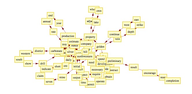
Graph of the Corpus generated by Closeness Centrality (has been plotted only the most relevant features)
Red color = high Closeness Centrality.
Purple = low Closeness Centrality.  

Results

There are three important things to highlight:

1. For this data set the TF-DF feature set returns the worst accuracy (the grain class TP = 43%) respect the other two methods.
2.  The TF – IDF and the Closeness Centrality give better results. And the accuracy is almost identical in absolute terms.
3.  The grain and oil classes are the tricky case: the algorithm is not able to divided them properly.

As you can imagine the third findings is the most important information returned by this experiment: it says us that we have to spend more efforts to highlight the differences among the classes oil and grain in order to increase the accuracy.

Notice that in the “TF - IDF” and “Closeness Centrality” the True Positive distribution is mirrored! This supports our thesis that we are not describing properly the documents belonging to these two classes.

We will see how to solve the problem!

Stay Tuned.

Feature Extraction - Different Approaches

When you build a classifier, and I'm not talking about only about the text categorization, you should have special care about this step.
If your features extractor has been made regardless the context,  whatever amazing classification algorithm you gonna use  ... the accuracy will be always unsatisfactory.
In the text categorization, you should  consider at least the following  points:

• document containing a lot of text or in opposite documents containing few words.
• document containing semantic  or in opposite documents without explicit semantic (like for example invoices or table)
• context dictionary: that is the set of words used in the domain your are working on (for example  words like acronyms having meaning only in a specific context)
• the overall environment where the classifier will work:  are there different languages? are there heterogeneous  sources? the manual classification is based only on the single document under processing?  
• business constraints: like max time to process a document or business process.

Bag Of Words based on  TF - (I)DF 

Term Frequency - Inverse document Frequency (TD IDF) function is based on a work of Spärck Jones and Karen in 1972. It basically combines local frequency property of a specific word in the document with a global property based on the number (inverse) of documents containing this word. Further technical details are available in internet (let me know if you are interested to the original paper published).

Even if this function is dated, we will show how to is it in smart way to achieve good accuracy.

• When does the TF DF work better than TF IDF?

When the documents of your domain contain few words (e.g. invoices,  spreadsheets, bank statements) the global component of IDF doesn't work well. In this context the easier TF DF works better!

In the classification sample we are working on, I gonna use K different Bag of Words (one bag of words  for each class) using both methods... we will check what is the best strategy!

To be honest I slightly modified the function in this way 

Modified TF (I)DF function

Where:

•  W_i[D_j] = Occurrences for the Word W_i in the document [D_j];
• DF[W_i] = Number of Documents containing  the Word W_i 
• |TrSet| = Number of Documents for the specific Class; 

The Features set has been obtained filtering the documents by the StopWord list and stemming each word considering only the "Base Form".

Here you are The first 20 Features extracted for the Reuters data Set TOPICS = "GOLD" (see the previous post for further details) with the respective weight:

TF DF			TF IDF
say	,51.907757725859135		sigma	,71.5899150352952
gold	,49.86505578380171		police	,64.30524039891371
ounce	,22.146187073000476		model	,64.30524039891371
ton	,8.317113808183201		land	,64.30524039891371
mine	,7.7300297803876585		grant	,64.30524039891371
company	,7.112820339974604		china	,64.30524039891371
pct	,7.094497045719568		pope	,64.30524039891371
year	,5.215953054827821		rand	,60.616126176742966
ore	,3.48549104848714		placer	,59.847379800543116
production	,3.2688965028783508		foot	,59.26642022035086
grade	,3.059411347433722		say	,58.04561519245233
silver	,2.5460893593153946		warrant	,57.23666647951021
price	,2.205337527517457		shoji	,55.38951920217253
reserve	,2.123335553835266		client	,55.38951920217253
drill	,2.118861548885319		ridge	,55.38951920217253
expect	,2.0390821784153337		alligator	,55.38951920217253
corp	,2.0390821784153337		play	,55.38951920217253
foot	,2.0236289512856094		vehicle	,55.38951920217253
short	,2.0225200886354586		grand	,55.38951920217253
average	,1.9028247115440413		action	,55.38951920217253

CLOSENESS CENTRALITY BASED

This is an attempt (I simplified a lot my the original version to highlight the main idea) using the Graph Theory to build a sort of "latent semantic" feature set.

After the filtering and stemming operations, I partitioned the document in couple of contiguous words and I built  a direct graph:

Sample of Direct Graph for a file of the Class "GOLD"

  To assign a score to a feature I used a Closeness Centrality function: The closeness centrality of a vertex u is defined as the inverse of the sum of the distance from u to all other vertices.

Assigning a color to the vertexes of the above graph (warm color for vertex having high score) you obtain:

Closeness Centrality assignment for the above graph

The first 20 features extracted using this method are:

bureau	,0.02127659574468085
interior	,0.01639344262295082
import	,0.014705882352941176
check	,0.01135161135161135
revise	,0.01105263157894737
technique	,0.01020408163265306
period	,0.00985400705790957
change	,0.009708737864077669
sigma	,0.009616273693943597
significant	,0.009615384615384616
cabinet	,0.009345794392523364
tunnel	,0.009212305611899932
affect	,0.008928571428571428
viceroy	,0.008796296296296295
conservatively	,0.008284833960972269
milling	,0.008240857798379922
practice	,0.008149473265752336
amenable	,0.008
cove	,0.0078125
department	,0.00757930926707298

How many Features Have we consider to obtain good accuracy?

How can we analyze the differences among the different Features Set seen before?

We will discuss about that in the next post.

Contact me at cristian.mesiano@gmail.com if you are interested to the Wolfram Mathematica source code.

Stay Tuned!!