Waiting Time Polynomials Document Classifier - Part III

Abstract
In the post is presented an innovative definition of polynomials associated to waiting time processes (analyzed in the former posts). Such polynomials are here  successfully used as document classifier. Comparative tests with SVM show significant accuracy improvements.

Boolean Classification tests based on test set of 8k randomly generated documents composed using an alphabet of three words.

Introduction
To encourage who found quite intricate the formula I presented a couple of posts ago, I'm going to present you an its practical application that might be a good incentive to analyze the formal aspects with more attention :)
What I show to you today is one of several application of such approach: a document classifier having higher accuracy than traditional methods as SVM (trained with gaussian kernel) and Neural Networks back propagated.

Characteristics of the classifier

• It's a supervised learning algorithm
• It's completely non parametric
• It can be used natively to classify multiple classes datasets.

The Algorithm
Let's assume to have a training set composed by two classes of documents: Cl_1, Cl_2.

    Learning Phase: Estimation of Geometrically distributed Random Variables.

1. Define an alphabet of three words {w1,w2,w3} using frequencies criteria or more sophisticated techniques.
2. For each class of training set:
• estimate parameters {p1, p2, p3} of the respective {X1(w1),X2(w2),X3(w3)} geometrically distributed random variables.
3. Calculate the polynomials associated to {X1(w1),X2(w2),X3(w3)} using:

    Testing Phase: document classification

1.  for each document Di of the test set:
• Identify the number of occurrences of  {w1,w2,w3}: {O_w1,O_w2,O_w3}
• Select the polynomial for which:
•  {O_w1,O_w2,O_w3} =p1^O_w1 p2^O_w2 p3^O_w3.
• Calculate the value of the polynomials P_Cl_1, P_Cl_2 using:
1. {p1, p2, p3} estimated for Cl_1
2. {p1, p2, p3} estimated for Cl_2
2. Classify the document:
1. If (P_Cl_1>P_Cl_2) Di belongs to Cl_1
2. Else Di belongs to Cl_2

Examples
1. How to select the polynomial

Let's consider the polynomials calculated using the aforementioned formula and assume that in document Di the word w1 is repeated 2 times, the word w2 is repeated 2 times and w3 is repeated 1 time.
Then, In the step 1 of the testing phase we have to choose the polynomial boxed in the below list:

Polynomials generated for O_w1+ O_w2+O_w3=5

2. Same polynomial, different values of  p1, p2, p3.

- How many polynomials are generated for O_w1+ O_w2+O_w3 = 25?

The answer is straightforward: 276 that is, all the possible configurations of 3 addends for which the sum =25. In the Encyclopedia of Integer Sequences, there are exciting explanation on such series.

- How does the polynomial change for different values of p1, p2, p3?

It's quite impressive how two polynomials can be different despite the setting of {p1, p2, p3} is almost identical.

Look at this example for which:

• On the left chart I plotted a polynomial with p1= 0.33, p2= 0.33, p3=0.34.
• On the right chart I plotted a polynomial with p1= 0.4, p2= 0.3, p3=0.3.

• In the first case the polynomial takes the maximum value for O_w1=8, O_w2= 8, O_w3 =9 ...not a big surprise!
• In the second case the polynomial takes the maximum value for O_w1=15, O_w2= 9, O_w3 =1. In this case the result is more complicated to be explained!

Document classification comparative test

To test the accuracy of my method I performed a comparative test using a randomly generated document set.

• The training set was composed by 100 documents (used to train a Gaussian Kernel SVM and to estimate params p_i for my method).
• The test set was composed by:
• Cl_1: 4000 documents randomly generated using a configuration of {p1, p2, p3}.
• Cl_2: 4000 documents randomly generated using a different configuration of {p1, p2, p3}.
• The accuracy has been tested using different configurations of {p1, p2, p3}, and considering different size of documents.

Results

First experiment: 

just the first 25 words have been considered  to estimate the params {p1, p2, p3}, to train the SVM and to test the the accuracy.

Accuracy results considering just the first 25 words.

Second experiment: 

Same test as above using the first 35 words of the documents.

Accuracy results considering just the first 35 words.

All the results showed there are referred to accuracy achieved on average using 10 different randomly generated test set and trying to configure SVM params to maximize the accuracy.

Considerations

As you can see the method based on definition of "Waiting Time Polynomials" that I'm proposing, performs significantly better than SVM.

More comparative tests will be shown in the publication I'm writing on such topic.

Further notes

Processes based on waiting time or geometrically distributed random variables are extremely important for risk assessment and risk evaluation.

I'll show you in another post some application of such polynomials in this field.

As usual, stay tuned

cristian

Document Classification: latent semantic vs bag of words. Who is the best?

We have seen few posts ago an approach to extract meta "concepts" from text based on latent semantic paradigm.
In this post we apply this approach to classify documents, and we do a comparison between this approach and the canonical bag of words.
The comparison test will be done through the ensemble method already showed in the last post.

Features
The idea is to build the features set considering constructs of co-occurrences instead of single words as usually done with bag of words.

• The prominent advantage of this approach is well rendered when the corpus contains structured features as for instance "bank account, invoice number" and so on. 
• The biggest disadvantage lays in the length of the feature set and consequently in the length of the vectors built to represent each document.

Let me clarify the last point: consider for instance a corpus of 100 words; in this case the dimension of each vectors will be less or equal to 100. Let's try now to consider the co-occurrences of these 100 words, and just to simplify the process, let's focus on the co-occurrences of two words (so we consider the closeness of two words), in this case the length of the vector is 100*100 =10000!!.

The image below represents the graph of the co-occurrences extracted considered the highest ranking (the ranking has been assigned in the way described in this post applied to the data set used to explain the ensemble method based on ADA boost M1).

The most important features extracted through the LSA method.

Vectors
To build the vectors I used the first 15000  structured features extracted by the latent semantic method and I considered just features composed by 2 words (co-occurrences).
To mitigate the complexity to crunch vectors with dimension so high, I built the training and test set using sparse matrixes of boolean values.
The advantage of the sparse matrix working with SVM is related to the small memory consumption required to select the support vectors.
Someone could argue that inner product of sparse array requires additional effort in the kernel evaluation, but if the vectors contain only boolean values, this extra complexity is negligible.

Comparison
To perform a comparison test, I used the same sets and the same strategies of learning.
In both scenarios, I trained the system through the ensemble techniques described in the last post (based on the boos method of ADA boost M1).

Results:
Before to discuss the results let me show the confusion matrixes.

Confusion Matrix for LSA based classifier.
(How to read it?...look at the former post)

Confusion Matrix for "Bag of Words" based classifier.
(How to read it?...look at the former post)

In blue it has been represented the results for LSA based approach.
In red it has been represented the results for Bag of Words approach.

As you can see, even if the results obtained with the LSA classifier are not so bad, the traditional approach based on bag of words (in this experiment extracted through TD-DF) returns better results.

Why?

The training set used generated around 8.000 features (single words) and the vectors have been built using 500 features (6.25% of the total). 

The size of the features having relevant ranking in the LSA approach is around 15000, and to ensure the same conditions of the test I trained the system choosing again 500 features (3.33% of the total).

Basically the useful information to classify the docs in LSA approach is spread over a bigger feature set.

Conclusion
As we have already seen in the past, doesn't exist a technique that perform better than other approaches with every data set. With this data set (a sub set of the Reuters 21578) the LSA requires more physical resources and returns worse results.

If we scratch the surface of the results, we can observe that it detects different aspects of the corpus to classify the docs: for instance it performs better with "GRAIN" category. So I wonder if we can take advantage of this aspect to ensemble this approach with the bag of words to improve further the accuracy (as suggested by a follower of this blog) !
...We will see the results of this conjecture the next post.
As usual: Stay Tuned!!
Cristian

Document Classification: how to boost your classifier

Time ago, we discussed about ADAboost as a meta algorithm useful to improve the accuracy of a weak classifier and I showed a sample on a boolean classification problem.
Frund and Schapire in this excellent paper proposed a version of this algorithm adapted to work with "multi labels" classifiers.

The two variants proposed in such paper are based on the trick to assign a weight to each sample of the training set in according with the error committed by the classifier, so it forces the classifier to be focused on the hard instances of the problem.
The improved classifier is finally obtained as a weighted combination of each version of the weak algorithm improved at each iteration.

Adaption of AdaBoost.M1 to a classifier SVM based.

ADaBoost.M1 tries to improve step by step the accuracy of the classifier analyzing its behavior on training set. (Of course you cannot try to improve the classifier working with the test set!!).
Here lays the problem, because if we choose as "weak algorithm" an SVM, we know that almost always it returns excellent accuracy on the training set with results closed to 100% (in term of true positive).
In this scenario, try to improve the accuracy of classifier assigning different weights to the training set doesn't work!

The idea of AdaBoost.M1 is still valid also with SVM classifiers, but I noticed that instead of to improve step by step the single SVM classifier,  we can train different SVM classifiers (with different parameters) and assign the score to each classifier based on the error committed on a part of the training set not used to train the SVM.
Let me explain better the procedure:

1. Split the training set in two different sets: training set (80% of the volume of the original training set), boosting set (20% of the volume of the original training set).
2. train k SVM classifiers with different parameters.
3. test the above SVM on the boosting set and calculate the beta score as done in the original implementation of ADAboost.M1.
4. The final answer of the boosted classifier is obtained as proposed by the original implementation of the Adaboost.M1

As you can notice, the method basically assigns to the k classifiers a "trustability score".


Real Case
Let's see what happens with our REUTERS-2158 data set:
I tried to classify the documents belonging to the categories: "GRAIN","CRUDE", "TRADE","OIL".
I trained four different SVM. Here you are what are the results of each classifier:

The Confusion Matrix for the Classifier I.The principal diagonal represents the True Positive.
In The circle the worst result for this classifier.

The Confusion Matrix for the Classifier II.The principal diagonal represents the True Positive.
In The circle the worst result for this classifier. 

The Confusion Matrix for the Classifier III.The principal diagonal represents the True Positive.
In The circle the worst result for this classifier. 

The Confusion Matrix for the Classifier IV.The principal diagonal represents the True Positive.
In The circle the worst result for this classifier. 

And after the application of the meta algorithm, here you are the confusion matrix for the improved classifier:

The Confusion Matrix for the Boosted classifier

As you can see the boosting provides us really good results! 

Here the same results showed in terms of precision and recall:

 

The Precision/Recall chart for the four weak classifiers.
(The ring shows the worst case for each classifier)

And here you are the Precision/Recall for the boosted classifier:

As usual Stay Tuned

Cristian

How the classifier accuracy is conditioned by the Feature Set (Bag of words)

In the last post we have seen a naïve approach to classify via SVM and C5, and we noticed that both SVM and C5 didn’t get good accuracy.

Despite the unsatisfactory results, we tested the different algorithms under the same conditions, and we found out that (at least in this case) they have the same behavior. Of course we should repeat the test in different conditions to provide a correct benchmark: in a next time we will do that.

But right now, I would like to perform a more useful (for our classification target) benchmark-test:

Consider an SVM based classifier, trained using the same parameters tuning strategy: How does the accuracy change if we build the vectors using different bag of words?

Basically we are trying to understand what is the best strategy to select the feature set (that is the bag of words) to classify our 4–classes data set.

Let me clarify immediately an important point:

• The strategy of “single bag of words” isn’t an approach really useful in real business scenarios: it is too much trivial.

So why are we doing such test?

Because these kind of tests can give us a lot of useful information about the data set, and allow us to choose the best strategy!

Test description.

We have already seen that measure the accuracy on the training set is extremely dangerous (soon or later I should explain the pillar of error theory and the overfitting problems…).

So the first step is to assess your experiment with a validation set (...there are more sophisticated test to do that like k-fold cross validation, but for our case should be enough): How can we do that?

…Easy: splitting the training set in two parts: the first one will be used to train the algorithm, and the second one will be used to measure the accuracy.

Be aware: you never can measure the accuracy using samples already observed by the learning algo. Of course you cannot measure the accuracy on the test set to retraining your system!! (please see the article of dr. Sandro Saitta at: http://www.dataminingblog.com/how-to-cheat-with-data-mining).

Training Set splitting

The second step is to build the vectors of the same training set using different bag of words. For this experiment, I used the “TF-DF”, “TF-IDF”, and the “Closeness Centrality” functions to extract the features and to build the vectors.

At this point we can assess the accuracy of the classifier with the same data set but built in different ways.

Accuracy test using TF-DF bag of words.
In the accuracy matrix (% format) the principal diagonal contains the true positive.  

Accuracy test using TF-IDF bag of words.
In the accuracy matrix (% format) the principal diagonal contains the true positive.

Accuracy test using Closeness Centrality based bag of words.
In the accuracy matrix (% format) the principal diagonal contains the true positive.  

The above tables shows (in percentage) the answers provided by the classifier (the diagonal are the True Positive). The element [i,j] = x says that: the real class was i and the classifier assigned to the class j x% of the documents belonging to i.

For the "graph theory based" bag of words, we can also shown the corpus distribution in terms of the closeness function:

Graph of the Corpus generated by Closeness Centrality (has been plotted only the most relevant features)
Red color = high Closeness Centrality.
Purple = low Closeness Centrality.  

Results

There are three important things to highlight:

1. For this data set the TF-DF feature set returns the worst accuracy (the grain class TP = 43%) respect the other two methods.
2.  The TF – IDF and the Closeness Centrality give better results. And the accuracy is almost identical in absolute terms.
3.  The grain and oil classes are the tricky case: the algorithm is not able to divided them properly.

As you can imagine the third findings is the most important information returned by this experiment: it says us that we have to spend more efforts to highlight the differences among the classes oil and grain in order to increase the accuracy.

Notice that in the “TF - IDF” and “Closeness Centrality” the True Positive distribution is mirrored! This supports our thesis that we are not describing properly the documents belonging to these two classes.

We will see how to solve the problem!

Stay Tuned.

Classification Step: C 5.0 vs SVM

Finally, after many preambles we have all conditions to classify the documents. So far we have seen:

1. How to translate a document in a vectors understandable by algorithms;
2. How to analyze the data set with density analysis;
3.  How to reduce the dimension of the problem (features reduction)

Well, now we have the all ingredients to classify the documents.

To show a couple of approach, I have extracted 4 classes from our REUTERS data set (choosing the criteria “TOPICS”, and considering the easier condition of documents belonging only to one class): “GOLD”,“GRAIN”,”OIL”,”TRADE”.

In this stage I put my self in a “comfortable zone” so, I considered the easiest way to classify the documents, that is, I built the vectors considering just ONE “bag of words”.

Basically I extracted the features set from the entire training set without any distinction of the specific class of the document.

In this approach we are delegating the entire complexity of the task to the classifier!

As we can see below, be lazy never pay!! (…I hope that it makes sense in English… ).

Let’s move on the results.

As I always recommend, never play with one toy! Be always curios and try different approach to solve the problem.

In this spirit for the time being I have done some tests using SVM (in LIBSVM implementation) and C.5 (the free version).

I embedded in Wolfram Mathematica the scripts to run both LIBSVM and C5 (contact me at cristian.mesiano@gmail.com if you desire the source); in this way all tasks (data preparing, features extraction, vector building and so on) can be done using only one interface.

Here you are the accuracy for SVM: 

Notice that the training set has been rescaled and weighted with different scores. 

Accuracy For SVM Classifier: Best results with Linear Kernel

As you can see, the accuracy measured on the training set is not brilliant! The OIL class is in the 50% of the case mislead. Moreover we have to consider that:

·      we are working with an easy data set and with few classes.

·      The accuracy has been measured only on the training set (…remember that the first error of the newbie is to focus much more on the training env.). The training set contains only points already observed by the classifier.  And analysis done only on it can hide overfitting problems!!

Even trying with different tuning, and with different kernels, the accuracy doesn’t improve.

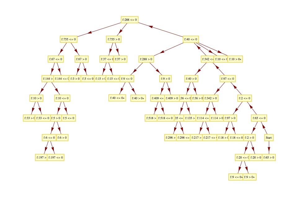
The situation doesn’t improve with C5: as you can see below, the accuracy is pretty much the same achieved via SVM.

The Decision Tree returned by C5 (plotted with Mathematica). 

Accuracy Matrix Provided by C5: The results are pretty similar to the SVM computations 

So Do we give up?

NEVER.

In the next posts we will see how improve the accuracy introducing boosting techniques.

…There are thousands of details to consider and to explain like:

linear kernels for SVM, how to measure the accuracy, how to improve the training set and avoid the over fitting…

We will see that in the next posts.

Stay Tuned

Cristian

SVM classification, an intuitive explanation and some test with LIBSVM

In a previous post I focused on linear classification and on the kernel trick to make linear separable points not linear separable.
...In this post I would explain why this trick is the base to build one of the most powerful classifier: the support vectors machines (SVM).
Consider the following set of point red and blue:

As you can see, you cannot find a straight line to divide blue points from the red points.
...But as mentioned before using the kernel trick we can find a space having greater dimension where these points can be separate by  straight line.
Formally,
we are looking for a  straight line

xi ·w+b≥+1 for yi =+1 and xi ·w+b≤−1 for yi =−1

where xi represents the points (blue or red), yi =+1 to represent red points and yi =−1for blue points.

w and b represent the unknown parameters of the straight lines.

The above equations can be combined into one set of inequalities: yi(xi ·w+b)−1≥0 ∀i

The SVM works out the classification bringing the points in a "kernel space" where the points can be divided finding a simple hyperplane.

I won't enter in technical details (the theory is based on Lagrange multipliers, kernel space, and Karush-Kuhn-Tucker Conditions) but if you are interested you can find an easy but exhaustive  description on "A Tutorial on Support Vector Machines for Pattern Recognition".

I implemented in Mathematica an easy routine to call the library LIBSVM to classify the above points (contact me to obtain the notebook):

To obtain this results (overall accuracy of classification: 99,2%) i trained the SVM using a gaussian kernel.

Another 2D sample (just to highlight the hyperplane I removed the color gradations):

2D points

Hyperplanes founds (in blue) for the above points

One of the interesting aspects of SVM is its vector notation: it allows a complete generalization of the problem: you can use the same algorithm to solve problem in any dimension!

For example in 3D scenario, you have:

3d Points 

Hyperplanes found

...another example:

Now we are ready to jump into the real world and attempt to classify text documents!

In the next post I will explain a real case application of document classification using SVM.

As usual: STAY TUNED!!

cristian

Linear classifier and non linear Classifier or rather: Input space and Feature Space

Sometimes during some meeting to explain a general classification problem I notice that many people don't understand the essential concept behind the classification.

In all fairness I discovered that many people confuse very often clustering with classification, but this is another story, and I promise to treat that in other post :).

What is the core concept to understand deeply the classification problem? ...the complexity of the problem itself!

Let me be more clear, and observe the following scenario:

Imagine that you are interested to divide the blue points from the red points, and more specifically you are interested to a black box taking in input a point, it is able to assign automatically the class (red or blue) to the point.

Well, Imagine that the only tool admitted to divide the plane to separate the points is the linear function.

Mhmm.... as you can see whatever line you try to draw is not able to split the points red from the blue points.

-> A linear function able to divide the plane splitting correctly the blue points from the red points is called linear classifier.

-> A non linear function able to that is called non linear classifier. (in this case the circle equation solve the problem.... but the real world is often more complex...)

Question: is it possible map the points of the original problem in another space more complex (that is having higher dimension) where is possible to divide the points using only a linear classifier?

The answer is YES. The trick is honor of famous mathematicians, but it is very very useful to make up a linear classifier (read easy to develop and easy to reuse in other context!!) and you can find the theory everywhere in internet.

Let me show the effect with the above problem:

I took every points in 2D and i mapped in 3D space using the function (called Kernel function): 

[x,y]->[x^2, Sqrt[2]*x*y, y^2]

And I obtained the following:

The red points now are grouped together and with a linear plane (that is a linear function in three dimensional space) we are able to divide again our points!

Here you are the overall problem:

If you are interested to further details I can share the Mathematica notebook I coded to generate the above images.

You don't need the License, you can play also with the player available here:http://www.wolfram.com/products/player/.

Let me cleanup the 10 rows of code and I'll publish the source file.

See you soon!

cristian