Text Clustering, a non parametric version of K-medoids algorithm for data de-duplication

Abstract
It's presented a quick and effective method to leverage text clustering for data de-duplication and normalisation.
The customised version proposed in this post bypasses the very well known problem of the assignment of the number of clusters.

Text Clustering results: each row depicts a cluster found. 

Introduction
One of the most common problems in the data management  is about the consistency: customer addresses, company names and whatever attribute in string format can be represented in multiple formats, often mutually equivalent.
Data normalisation presents some challenges, especially in the following scenarios:

• Variations/mutation of the trusted source of information are not a priori known.
• The data to be normalised are characterised by high volume.
• There are no deterministic and static rules to normalise the data.
• ...you don't have plenty time to find the perfect solution :), and you have to deliver fast!

Why the brute force approach it's wasted time!
Let's assume that you already found for your specific use case the best distance to judge how far is a record  from another one.
To make the story a bit more realistic, let's assume hereafter that our attribute to be normalised is a string.
...I would hope that nobody of you really thought to create a big matrix to keep track of the all possible distances among the possible values of the attribute... Why? If you have for instance 10k possible values, you need to computate at least 49.995.000 comparison (assuming that your distance is symmetric!), that's because the complexity follows Binomial[N,2].
You might perform the brute force approach over a statistically representetive sample set, but in that case it's really hard the validation of the real accuracy of your results.

Why Partitional Clustering is efficient?
As you know, this is a "practical mean" blog, so I encourage you to refer to real books if you are looking for the theoretical proof. Anyhow it's easy to get convinced about the following:

• number of comparisons to be performed assuming $K$ clusters, $I$ iterations, $N$ elements to be clustered: $N \cdot K \cdot I$.
• number of comparison to update the centroids: $I \cdot (\binom{K_1}{2}+\binom{K_2}{2}+\cdots+\binom{K_K}{2}) << \binom{N}{2}$

The comparison of the computational complexity of the brute force approach with the partitional clustering is well depicted by the below example, where I assumed ten iterations to get the convergence, 10 clusters, a data set that grows from 1000 to 20.000 points:

The computational effort: in red the  brute force approach, in blue the clustering.

The approach in a nutshell 

1. Group together records that look similar each other using k-medoid clustering 

2. Store in a index the centroids found.

3. delete (only if the use case allows it) all the member of the clusters with exception of the centroids.

4. for each new record to be stored in the DB, perform the comparison with the elements of the index: if the distance is to high, add the new record to the index.

K-medoids vs K-means

The main difference of K-medoid respect the well known K-means is in the assignment of the centroids:

• in K-means the centroid is the barycenter of the cluster, so it might not be a real record.
• in K-medoids, the centroid is a record of the cluster that minimises the sum of the distances respect all the other points of the cluster. Of course, depending on the case, you might prefer minimise the variance, or even define more sophisticated minimisation criteria.
• K-means is usually much faster, since the computation of the barycenter it's usually taken as average of the position of the records in the space,
• K-medoids requires (for each cluster) the additional comparison of the distances of the points of the cluster from all the other points of the clusters (that explains the formula mentioned in the complexity formula.

K-medoids is more robust than k-means in the presence of noise and outliers.

...But there is still something that makes me unhappy with K-medoids: It's parametric, meaning it requires the priori knowledge of the number of clusters.

In the real world simply forget it! 

Customised version for auto-determination of number of clusters.

1. Instantiate the standard k-medoids with arbitrary number of classes (in the case analysed later I used just two clusters as initialisation).
2. after the operation to update the medoids,  compare the medoids with the others: if two medois are very similar, then merge the two clusters.
3. calculate the mean distances (this computation can take advantages of the operations performed during the medoids updating) for each cluster: if the mean distance overcome a threshold (that indicates the sparsity of the points of the cluster) then split the cluster. In this experiment I used a wild approach: each point of the split cluster have been consider as new cluster.
4. goto step 2 until convergence. 

You might argue that such customisation doesn't require the "number of cluster" as param but introduce two thresholds: one for the clustering merging and another one for the splitting.
Actually the threshold is just one:

• if $\theta$ is the minimum acceptable distance for which two strings might be considered as the same, then $1- \theta$ is the threshold for which two strings are absolutely different!

The advantage of the approach lyes on the fact the estimation of the threshold can be easily estimated and verified. The estimation of #clusters it's not that easy!

Experiment: Addresses de-duplication.
As data set I downloaded from this link the addressees of the pizzeria in New York (I'm Italian, and I love pizza :D).
To assess the accuracy of the algorithm I randomised each entry introducing a gaussian noise.

Data Perturbation:
The perturbation method I used, is based on randomised swapping of characters of the string:

1. Select the number $n$ of characters you want to swap. Such number is drawn within the range [0,StringLength[str]] using a gaussian distribution.
2. Draw $n$ couples of integers (between[1,StringLength[str]]).
3. For each couple swap the corresponding first character with the second.

Distance
The definition of distance is crucial: several options are available. In this experiment I used the common Nedelman-Wunsch similarity. I'm pretty sure that good results can be achieved also with Jaro-Winkler and Levenshtein distances.

Experiment Setting
I firstly estimated the param of the customised k-medoid algo: the Merging/Splitting threshold.
The value is dependent by the nature of the data.

• What's the minimum acceptable distance between two strings to be considered the same?

I selected randomly several couples of strings, measured the distances and sorted by value.
I noticed that 70% of matching it's the good one.
In the next posts I'll show a technique more refined based on the convergence slope of the clustering... but that's another story.

Results:
The data set contains 50 records:

• 10 different addresses
•  for each address 5 deviations generated with the aforementioned perturbation.

The customised K-medoids found the best result (that is 10 clusters containing the 5 deviated addresses) ~20% of the cases (first bar of the below chart)
The below chart shows how many time (out of 100 trials) the alto found exactly $k$ number of clusters.

The first bar says that 22 times out 100 trials, the alto returned 10 clusters.

• As you can see, in 70% of the cases the algorithm partitions the data set in [9,12] clusters!

Below the best and worst case

Best case: achieved 20% of the cases. Steps to converge ~26.  

Worst case: returned 17 clusters. Convergence after 40 steps.

Convergence of the algorithm:
The time to converge is the following:

• On average the algorithm converges after 36 steps.

I noticed that longer is time to converge, lower is the probability to determine correctly the number of clusters.

As usual: stay tuned!
cristian

Clustering algorithm to approximate functions

In the last post we discussed about function approximation through polynomials having exponents in the Real domain.
We have also seen that to obtain a good approximation of the function, long training session is required; the reason of this inefficiency lays in one and on the gradient surface and in another hand on the strategy adopted to train the system.
Let me spend few words about the gradient surface:

The gradient surface conformation is strictly related with the number of monomials used to approximate functions, so

• if you use fews monomials the approximation cannot be good because you are using less complexity respect the complexity of the original function and the gradient will have pretty regular convex surface with bottom equal to best approximation achievable by the linear combination of monomials chosen.
• if you use too many monomials, you are building a complex gradient function (because the number of its parameters are growing), so you increase the risk to fall down in a local minimum.

I mentioned that annealing strategy can help to overcome the barriers imposed by local minimums, but for the time being I prefer show you a little bit more sophisticated strategy: the clustering learning.
As you know usually the clustering techniques are used to divide data in different categories, but I would like once again deliver the message that in data mining (and in text mining as well) what is real important is not the product, the tool or the suite, but the knowledge, the creativity and the skills to abstract the problems and the algorithms and adapt the second one to solve the first one.

Divide et Impera (Latin motto)
... that is divide the problem in sub problems, find sub solutions and merge them to obtain the overall solution.
The strategy is very easy to describe:
1. Divide the domain of your function in k sub intervals.
2. Initialize k monomials;
3. Consider the monomials as centroids of your clustering algorithm.
4. Assign the points of the function to each monomial in compliance to the cluster algo.
5. Use the gradient descent to adjust the parameters of each monomial.
6. Go to 4. until the accuracy is good enough.

Basically in the former version we had this approximation:

Function Approximation through power real polynomials

While in this approach we introduce the membership of function which assign each point to each cluster (in this case monomial)

Power Real Polynomials approximation with clustering approach

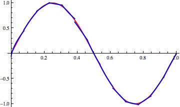
Let's see the result obtained with the sinusoid function (please compare with the former results obtained with the canonical gradient descent).

Clustering approach to fit the Sin(x) function

Let me show how these strategy works in more complex domains, for example in R^3 (of course you should add extra "y" variable to the monomial).
First Example

And here you are the monomials found and the fitting found applying the membership function (I choose a crispy version but it is also feasible a fuzzy approach):

The spheres represent the points belonging to the original function, while the planes are representing the monomials surface found by clustering & gradient. (approximation with 36 monomials)

And the fitting obtained:

Original Function depicted with  blue points; Fitting depicted with Orange Points  

Second Example
The function chosen is the following:

On the left side the original function,
 on the right side the hyperplanes (monomials) found by gradient descent cluster based.

The fitting obtained applying the above monomials and the membership function:

The graphs shows the plane described by the original function.
In blue the  points belonging to the original function.
In orange the fitting obtained using the clustering based procedure.

As usual: Stay Tuned 

Cristian

Support Vector Clustering: An approach to overcome the limits of K-means

Time ago, I posted a banal case to show the limits of K-mean clustering. A follower gave us a grid of different clustering techniques (calling internal routines of Mathematica) to solve the case discussed.
As you know, I like write by myself the algorithms and I like show alternative paths, so I've decided to explain a powerful clustering algorithm based on the SVM.
To understand the theory behind of SVC (support vector clustering) I strongly recommend  to have a look at: http://jmlr.csail.mit.edu/papers/volume2/horn01a/rev1/horn01ar1.pdf . In this paper you will find all technical details explained with extremely clearness.
As usual I leave the theory to the books and I jump into the pragmatism of the real world.
Consider the problem of a set of points having an ellipsoid distribution: we have seen in the past that K-means doesn't work in this scenario, and even trying different tweaks changing the position of the centroids and its number of centroids, the final result is always unacceptable.
SVC is a clustering algorithm that takes in input just two parameters (C and q) both of them real numbers. C is to manage the outliers and q is to manage the number of clusters. Be aware that q is not directly related with the number of clusters!! Tuning q  you can manage the "cluster granularity" but you cannot decide a priori the number of clusters returned by the algo.


How to implement SVC.
There are many implementations of SVC, but I would like to show different tools (I love broaden the horizons...), so the ingredients of the daily recipe are: AMPL & SNOPT.
Both of them are commercial tools but to play with small set of points (no more than 300) you can use for free the student license!
AMPL is a comprehensive and powerful algebraic modeling language for linear and nonlinear optimization problems, in discrete or continuous variables and SNOPT is a software package for solving large-scale optimization problems (linear and nonlinear programs).
AMPL allows the user to write the convex problem associated to SVC's problem in easy way:

The AMPL file for SVC

And SNOPT is one of the many solvers ables to work with AMPL.

In the former image, after the statement "param x: 1  2   3   :=" there are the list of 3D points belonging to our data set.

One of the characteristics of SVC is the vector notation: it allows to work with high dimensions without changes in the development of the algorithm.

2D Problem 
Let's show the application of SVC in our ellipsoid data set

300 pt having ellipsoid distribution.  The first contour of SVC  has been depicted in black.   

The above image shows the clusters (depicted like connected components of a graph...read further details in the mentioned paper) returned by SVC and plotted by Mathematica.

3D problem
Just to show the same algorithm working in 3D on the same problem:

3D points having ellipsoid distribution.

And Here you are the SVC results plotted by Mathematica:

SVC applied on the former data set

As you can see in both scenarios SVC is able to solve the easy  problem that K means cannot manage.

PS

We will continue the text categorization in the next post... From time to time I allow to myself some divagation. 

Kmeans: an easy clustering algorithm... maybe too easy for real world problems

I was writing the first post about the document auto classification, when a friend contacted me for an opinion related to clustering algorithm.
I had a quick look at the dataset (4 components, I plotted the four combinations of 3D subsets, and I saw that the shapes were pretty much like an ellipsoid).
Let me report the call:
me:"what kind of clustering algorithm did you use?"
him: "k-means!"
me: "the stupid k-means?"
him: "yes, the data set is pretty much regular and the points are well divided so I believe kmeans should work properly...Do you think I made a mistake to implement it?"
me: "no you are a fantastic developer. More easily it cannot work with data organized like ellipsoid shape! ...try to visit wikipedia, there is a nice sample with iris data set to explain where it fails"
him: "but iris data set is a tricky set, the points are overlapped, my scenario is different: it is more easy!".
me: "ok, this evening visit my blog, I'll show you a nice sample where the data are definitely divided, but the kmeans fails!"

Two set of points,  in different colors the clusters obtained, the two big points are the centroids.

Just to have another prospective, I have done the same test in 3D:

Two set of points,  in different colors the clusters obtained, the two big points are the centroids.

Of course, increasing the number of centroids, the situation gets worse and worse:

I really hope that my dear friend will be convinced that doesn't exist an algorithm useful for all kind of problem!
Moreover... I would have in my job dataset "tricky" like Iris!!!
Contact me for the notebook to play with the simulations.

Stay Tuned.

PS: I'll be on vacation until the end of the month... see you soon!