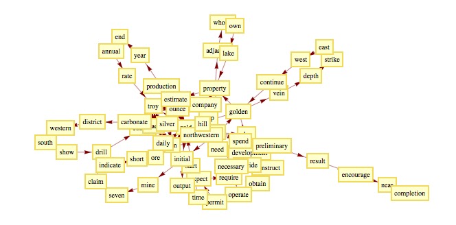
Wednesday, August 17, 2011

Build the vectors and Feature Reduction

Part I: building the vectors
In the former post we have created a features set for the class GOLD, now we show how use this features set to build the vectors to feed the svm.
The Features set is the fingerprint that characterizes the document class.
To build the vectors, you have to follow the same parsing and filtering process used to extract the features.
As described in the previous post,  from the original file, you have to follow the below steps:
  • Split the words of the file;
  • Remove the words having Length <= 2;
  • Remove the stopWords
  • Take the "root" of the word (e.g. Large from Larger)
On the filtered file just obtained, you can build every sort of statistic to associate to each word of the filtered file a score.
For our purpose the simple frequency could be enough.
 The last step is to associate to each word of the filtered file the score just calculated with the score associated to each word of the features set.
This step is illustrated in the below illustration:
"FT score" stands for Feature set score, < . , . > stands for a linear operator.
Notice that a vector assumes 0 value when the filtered file doesn't contain occurrences for the specific feature.
The grey box is the final Real Number vector. 
As you can see the vector has the same dimension of the Feature Set, in this case (built using TF-DF) it has dimension equal closed to 1000.
In a enterprise environment it could be a bottleneck in terms of computational capabilities, this due to the strict relation between vector dimension and time complexity to classify.

Part II: reducing the dimension
How can we reduce the dimension of the problem to speed up the entire classification process?
There are different methods,  the first I would show is the Principal Component Analysis (PCA).
As usual, I'm not going to enter in technical and theoretical issues: there are thousands websites, tutorial and paper  where you can find every sort of details on that.
Just to have an overview, PCA provides the most important linear components in a set of data. It is based on the concept of eigenvectors and eigenvalues : M.x = λ x where λ is the eigenvalue and x is the eigenvector.
PCA has two great features:
  1. it is completely unparameterized;
  2. it is extremely easy to implement; 
In Mathematica the implementation takes no more than 4-5 rows code:

the variable matrix is the dataset having whatever Dimension

Basically you standardize the data (to have mean = 0),  you compute the covariance matrix, and on that you extract the eigenvalues and eigenvectors.
The position of eigenvectors having higher eigenvalues are the the component most relevant: the components relevant are the features most important to classify the documents with a minimum loss of accuracy!
Just to understand the role played by eigenvectors consider  the following multivariate gaussian data set:

Data set gaussian distributed

The principal components are well represented by the red vectors:
Principal Components for the above data set 
Nevertheless, PCA is not useful in data having different density, and before to discard components (features) from your data set, I suggest to analyze the density!

What happens in our classes? 
I computed the PCA for the GOLD class, but the question  now is "What is the minimum threshold to discriminate the important components against the negligible features?   
...Sometimes a simple "logPlot" helps the analyst:

The blu arrow represent the discontinuity point for the eigenvalues 
As shown above, around at the component number 82, there is a discontinuity: after this point the magnitude of the eigenvalue is negligible. Here you are the threshold! 
Remark
The vectors have been built using the sorted Feature Set list (see the previous post).
and the criteria to sort was based on the TF- DF (or TF IDF, or ...): from the most important from TF DF prospective to the less important.
The graph above provides us a sort of countercheck of the goodness of the criteria chosen to select the features, because there is a perfect correspondence among the weight assigned with TF DF and the eigenvalues (notice the monotonicity of the graph)!
So for the GOLD class, we will consider only the first 82 components.
As you can see we used PCA in two different ways:
1) to countercheck our features extraction method
2) to reduce the complexity of the problem from 1000 to 82.

In the next post, we will see another algorithm of feature reduction: C4.5.
...We are now introducing many different approaches to play with the data, in the next post I'll show you the graph of experiments we are doing to keep track of every results and to chose the best strategy.
as usual: stay tuned
cristian

Tuesday, August 9, 2011

Feature Extraction - Different Approaches

When you build a classifier, and I'm not talking about only about the text categorization, you should have special care about this step.
If your features extractor has been made regardless the context,  whatever amazing classification algorithm you gonna use  ... the accuracy will be always unsatisfactory.
In the text categorization, you should  consider at least the following  points:
  • document containing a lot of text or in opposite documents containing few words.
  • document containing semantic  or in opposite documents without explicit semantic (like for example invoices or table)
  • context dictionary: that is the set of words used in the domain your are working on (for example  words like acronyms having meaning only in a specific context)
  • the overall environment where the classifier will work:  are there different languages? are there heterogeneous  sources? the manual classification is based only on the single document under processing?  
  • business constraints: like max time to process a document or business process.
Bag Of Words based on  TF - (I)DF 
Term Frequency - Inverse document Frequency (TD IDF) function is based on a work of Spärck Jones and Karen in 1972. It basically combines local frequency property of a specific word in the document with a global property based on the number (inverse) of documents containing this word. Further technical details are available in internet (let me know if you are interested to the original paper published).
Even if this function is dated, we will show how to is it in smart way to achieve good accuracy.
  • When does the TF DF work better than TF IDF?
When the documents of your domain contain few words (e.g. invoices,  spreadsheets, bank statements) the global component of IDF doesn't work well. In this context the easier TF DF works better!

In the classification sample we are working on, I gonna use K different Bag of Words (one bag of words  for each class) using both methods... we will check what is the best strategy!
To be honest I slightly modified the function in this way 

Modified TF (I)DF function
Where:
  •  W_i[D_j] = Occurrences for the Word W_i in the document [D_j];
  • DF[W_i] = Number of Documents containing  the Word W_i 
  • |TrSet| = Number of Documents for the specific Class; 
The Features set has been obtained filtering the documents by the StopWord list and stemming each word considering only the "Base Form".
Here you are The first 20 Features extracted for the Reuters data Set TOPICS = "GOLD" (see the previous post for further details) with the respective weight:

             TF DF                TF IDF
say ,51.907757725859135 sigma ,71.5899150352952
gold ,49.86505578380171 police ,64.30524039891371
ounce ,22.146187073000476 model ,64.30524039891371
ton ,8.317113808183201 land ,64.30524039891371
mine ,7.7300297803876585 grant ,64.30524039891371
company ,7.112820339974604 china ,64.30524039891371
pct ,7.094497045719568 pope ,64.30524039891371
year ,5.215953054827821 rand ,60.616126176742966
ore ,3.48549104848714 placer ,59.847379800543116
production ,3.2688965028783508 foot ,59.26642022035086
grade ,3.059411347433722 say ,58.04561519245233
silver ,2.5460893593153946 warrant ,57.23666647951021
price ,2.205337527517457 shoji ,55.38951920217253
reserve ,2.123335553835266 client ,55.38951920217253
drill ,2.118861548885319 ridge ,55.38951920217253
expect ,2.0390821784153337 alligator ,55.38951920217253
corp ,2.0390821784153337 play ,55.38951920217253
foot ,2.0236289512856094 vehicle ,55.38951920217253
short ,2.0225200886354586 grand ,55.38951920217253
average ,1.9028247115440413 action ,55.38951920217253

CLOSENESS CENTRALITY BASED
This is an attempt (I simplified a lot my the original version to highlight the main idea) using the Graph Theory to build a sort of "latent semantic" feature set.
After the filtering and stemming operations, I partitioned the document in couple of contiguous words and I built  a direct graph:
Sample of Direct Graph for a file of the Class "GOLD"
  To assign a score to a feature I used a Closeness Centrality function: The closeness centrality of a vertex u is defined as the inverse of the sum of the distance from u to all other vertices.
Assigning a color to the vertexes of the above graph (warm color for vertex having high score) you obtain:
Closeness Centrality assignment for the above graph

The first 20 features extracted using this method are:
bureau ,0.02127659574468085
interior ,0.01639344262295082
import ,0.014705882352941176
check ,0.01135161135161135
revise ,0.01105263157894737
technique ,0.01020408163265306
period ,0.00985400705790957
change ,0.009708737864077669
sigma ,0.009616273693943597
significant ,0.009615384615384616
cabinet ,0.009345794392523364
tunnel ,0.009212305611899932
affect ,0.008928571428571428
viceroy ,0.008796296296296295
conservatively ,0.008284833960972269
milling ,0.008240857798379922
practice ,0.008149473265752336
amenable ,0.008
cove ,0.0078125
department ,0.00757930926707298
How many Features Have we consider to obtain good accuracy?
How can we analyze the differences among the different Features Set seen before?
We will discuss about that in the next post.
Contact me at cristian.mesiano@gmail.com if you are interested to the Wolfram Mathematica source code.
Stay Tuned!!

Tuesday, August 2, 2011

Document Classification part 1 - Data Set Analysis

As promised, in this post I'm going to discuss about an important branch of text analytics: the text categorization.
Step by step, we will build a classifier going through the following steps:

  • Data set preparing.
  • feature extraction.
  • feature reduction comparing different techniques like PCA, C4.5, and other algos.
  • Translation of the documents in the proper form to feed the classification algorithms.
  • Classification via SVM ...we will explore different strategies to adapt a boolean classifier to multi class algorithm 
  • Benchmarking with other classifiers like C4.5, naive Bayes Classifier.
As you can see, it will take plenty time to show every method, and I really hope you will attend proactively to exchange experiences.

After the pcreambolus, let's start with the first step: "data set preparing".
I decided to use for this experiment a very common standard data set: the Reuters-21578 data set.
It is a data set often used in academical context to perform benchmark tests over different strategies. 
It is organized in tagged files (sgm) easy to handle to build ad hoc data set, and you can download it at: http://www.daviddlewis.com/resources/testcollections/

Here you are the composition of the data set:
The Reuters-21578 data set composition
As you can see it is a multi dimensional data set, that is you can perform classification tasks across different kind of categories.
For example, you could build a data set considering "TOPICS" classes where "PLACES" = "Canada" and so on.
For our tests I decided to work with categories TOPICS: there are documents belonging to 135 different classes of TOPICS.
In a realistic scenario (by enterprise prospective) build an efficient classifier for 135 classes is too much expensive in terms of efforts to achieve good accuracy for each class, in terms of maintenance, and in terms of computational efforts.
So, if there aren't business constraints, is important perform a quantitative analysis to detect which are the most common classes.

The most important classes for "TOPICS" categories
The important question is:
How many classes have I to consider to cover at least X% of the entire amount of documents?
x- axis = classes (sorted by volume) --- y-axis % of documents covered 
As you can see, considering for example only 20 classes instead of 135, we are able to cover around 80% of all documents in the data set: this is the "Pareto Principle"!

If you are interested to play with the Reuters data set and follow the step by step classifier building, I arranged a Wolfram Mathematica notebook to extract automatically training/test set, using custom categories. Contact me directly at cristian.mesiano@gmail.com

Wednesday, July 13, 2011

Kmeans: an easy clustering algorithm... maybe too easy for real world problems

I was writing the first post about the document auto classification, when a friend contacted me for an opinion related to clustering algorithm.
I had a quick look at the dataset (4 components, I plotted the four combinations of 3D subsets, and I saw that the shapes were pretty much like an ellipsoid).
Let me report the call:
me:"what kind of clustering algorithm did you use?"
him: "k-means!"
me: "the stupid k-means?"
him: "yes, the data set is pretty much regular and the points are well divided so I believe kmeans should work properly...Do you think I made a mistake to implement it?"
me: "no you are a fantastic developer. More easily it cannot work with data organized like ellipsoid shape! ...try to visit wikipedia, there is a nice sample with iris data set to explain where it fails"
him: "but iris data set is a tricky set, the points are overlapped, my scenario is different: it is more easy!".
me: "ok, this evening visit my blog, I'll show you a nice sample where the data are definitely divided, but the kmeans fails!"
Two set of points,  in different colors the clusters obtained, the two big points are the centroids.
Just to have another prospective, I have done the same test in 3D:


Two set of points,  in different colors the clusters obtained, the two big points are the centroids.
Of course, increasing the number of centroids, the situation gets worse and worse:
I really hope that my dear friend will be convinced that doesn't exist an algorithm useful for all kind of problem!
Moreover... I would have in my job dataset "tricky" like Iris!!!
Contact me for the notebook to play with the simulations.
Stay Tuned.
PS: I'll be on vacation until the end of the month... see you soon!


Thursday, July 7, 2011

SVM classification, an intuitive explanation and some test with LIBSVM

In a previous post I focused on linear classification and on the kernel trick to make linear separable points not linear separable.
...In this post I would explain why this trick is the base to build one of the most powerful classifier: the support vectors machines (SVM).
Consider the following set of point red and blue:

As you can see, you cannot find a straight line to divide blue points from the red points.
...But as mentioned before using the kernel trick we can find a space having greater dimension where these points can be separate by  straight line.
Formally,
we are looking for a  straight line

xi ·w+b≥+1 for yi =+1 and xi ·w+b≤−1 for yi =−1
where xi represents the points (blue or red), yi =+1 to represent red points and yi =−1for blue points.
w and b represent the unknown parameters of the straight lines.
The above equations can be combined into one set of inequalities: yi(xi ·w+b)−1≥0 ∀i
The SVM works out the classification bringing the points in a "kernel space" where the points can be divided finding a simple hyperplane.
I won't enter in technical details (the theory is based on Lagrange multipliers, kernel space, and Karush-Kuhn-Tucker Conditions) but if you are interested you can find an easy but exhaustive  description on "A Tutorial on Support Vector Machines for Pattern Recognition".
I implemented in Mathematica an easy routine to call the library LIBSVM to classify the above points (contact me to obtain the notebook):
To obtain this results (overall accuracy of classification: 99,2%) i trained the SVM using a gaussian kernel.
Another 2D sample (just to highlight the hyperplane I removed the color gradations):

2D points
Hyperplanes founds (in blue) for the above points


One of the interesting aspects of SVM is its vector notation: it allows a complete generalization of the problem: you can use the same algorithm to solve problem in any dimension!
For example in 3D scenario, you have:


3d Points 
Hyperplanes found


...another example:


Now we are ready to jump into the real world and attempt to classify text documents!
In the next post I will explain a real case application of document classification using SVM.
As usual: STAY TUNED!!
cristian

Thursday, June 30, 2011

Full text search engines competition: ... the winner is... the stupid "occurrences counter"!!

I was reading some technical features on full text search engines.
To be honest I'm not an expert on this kind of technology, but I saw that it is very easy impress people with astonishing announcements like:
"forget the occurrences, it is time of concepts; our engine is able to really understand the meaning of the key search!".
Wow! At the glance seems that these engines are able to order autonomously a pizza with out any human interaction.
But. ...there is alway a "but":
1) is it always the best solution a "semantic seeker"?
2) is it so complex build a customer solution starting from our old search engine?
Well. For the first point my opinion is that for each domain exists a specific solution. For example if the set of documents indexed in your docbase is mainly composed by invoices, or table documents (like spreadsheets) or advice for new orders, I don't see many advantages using semantic engine.
May be for documents containing many phrases and free text, this kind of technology could bring some added value. ...But I would like to see some honest benchmark on that.
Even for the classification problem is not yet proved that a semantic classifier works better a unstructured  classifier (I'll arrange a post on that with some real test!).
For the second point.... the only way to check it is.... to try!
So let start with a stupid key search like "turbojet airplane"
Our old full text search engine (FTSE) will retrieve docs containing both "turbojet" and "airplane".
we could enrich with our specific (business) requirements!
For Example, using many different dictionaries available in internet I arranged a recursive (2 loops) lookup on the first set of "synonyms" (extend in this trivial example with broader terms and morphological derivatives terms). After that I built the graph of the connections and to restrict the set of pertinent terms i clustered the graph using a stupid k-means.  The final list of words is selected choosing the cluster containing the original word! ...No more chatting:
for the word "turbojet" the set of words to enrich our old FTSE is:
The cluster of words selected is painted in orange

and for the word "airplane":
Even in this case i painted the selected cluster of words in orange.
The method is very general and tunable because:
1) you can select or deselect you preferred dictionaries (depending on your data domain),  
2) you can enrich/impoverish the set of words tuning the number of loops for the recursive search.
3) you can choose different clusters
Of course the latest FTSE are faster and the sophisticated, but we can extend the life of our old engine with few maintenance.
I love simplicity :) ...occam's razor.
cristian

Cristian welcomes you to our blog!

Hi All,
... Sorry, but it is my first blog... and I forgot to introduce my self... 
I'm Cristian, an italian guy employed in a big multinational company in Zürich. As you will see, my English is pretty terrible despite I'm working on Text Mining projects in the Content Management department of my company :).
I really hope you will correct my mistakes... (the trial error strategy is a good paradigm to train many systems: also human brains to learn quickly foreign languages!!).
My contributes to this blog will be mainly summarized in three points:
1) specialization of general purpose algorithms;
2) visual example of real scenarios;
3) analysis of systems (understood as mix of cooperative algorithms) for complex problems.
Of course we get the focus on text mining and data mining problem, but as you know many techniques are so general that you can easily reuse in different context.
Our interests in the last years have been oriented on problems related to content auto classification, extraction of relevant information from text, and selective search enforcing standard capabilities of "full text search engine".
If you are attracted  to these themes and you want share with us your experiences and points of view, well: STAY TUNED!