Waiting Time Polynomials Document Classifier - Part III

Abstract
In the post is presented an innovative definition of polynomials associated to waiting time processes (analyzed in the former posts). Such polynomials are here  successfully used as document classifier. Comparative tests with SVM show significant accuracy improvements.

Boolean Classification tests based on test set of 8k randomly generated documents composed using an alphabet of three words.

Introduction
To encourage who found quite intricate the formula I presented a couple of posts ago, I'm going to present you an its practical application that might be a good incentive to analyze the formal aspects with more attention :)
What I show to you today is one of several application of such approach: a document classifier having higher accuracy than traditional methods as SVM (trained with gaussian kernel) and Neural Networks back propagated.

Characteristics of the classifier

• It's a supervised learning algorithm
• It's completely non parametric
• It can be used natively to classify multiple classes datasets.

The Algorithm
Let's assume to have a training set composed by two classes of documents: Cl_1, Cl_2.

    Learning Phase: Estimation of Geometrically distributed Random Variables.

1. Define an alphabet of three words {w1,w2,w3} using frequencies criteria or more sophisticated techniques.
2. For each class of training set:
• estimate parameters {p1, p2, p3} of the respective {X1(w1),X2(w2),X3(w3)} geometrically distributed random variables.
3. Calculate the polynomials associated to {X1(w1),X2(w2),X3(w3)} using:

    Testing Phase: document classification

1.  for each document Di of the test set:
• Identify the number of occurrences of  {w1,w2,w3}: {O_w1,O_w2,O_w3}
• Select the polynomial for which:
•  {O_w1,O_w2,O_w3} =p1^O_w1 p2^O_w2 p3^O_w3.
• Calculate the value of the polynomials P_Cl_1, P_Cl_2 using:
1. {p1, p2, p3} estimated for Cl_1
2. {p1, p2, p3} estimated for Cl_2
2. Classify the document:
1. If (P_Cl_1>P_Cl_2) Di belongs to Cl_1
2. Else Di belongs to Cl_2

Examples
1. How to select the polynomial

Let's consider the polynomials calculated using the aforementioned formula and assume that in document Di the word w1 is repeated 2 times, the word w2 is repeated 2 times and w3 is repeated 1 time.
Then, In the step 1 of the testing phase we have to choose the polynomial boxed in the below list:

Polynomials generated for O_w1+ O_w2+O_w3=5

2. Same polynomial, different values of  p1, p2, p3.

- How many polynomials are generated for O_w1+ O_w2+O_w3 = 25?

The answer is straightforward: 276 that is, all the possible configurations of 3 addends for which the sum =25. In the Encyclopedia of Integer Sequences, there are exciting explanation on such series.

- How does the polynomial change for different values of p1, p2, p3?

It's quite impressive how two polynomials can be different despite the setting of {p1, p2, p3} is almost identical.

Look at this example for which:

• On the left chart I plotted a polynomial with p1= 0.33, p2= 0.33, p3=0.34.
• On the right chart I plotted a polynomial with p1= 0.4, p2= 0.3, p3=0.3.

• In the first case the polynomial takes the maximum value for O_w1=8, O_w2= 8, O_w3 =9 ...not a big surprise!
• In the second case the polynomial takes the maximum value for O_w1=15, O_w2= 9, O_w3 =1. In this case the result is more complicated to be explained!

Document classification comparative test

To test the accuracy of my method I performed a comparative test using a randomly generated document set.

• The training set was composed by 100 documents (used to train a Gaussian Kernel SVM and to estimate params p_i for my method).
• The test set was composed by:
• Cl_1: 4000 documents randomly generated using a configuration of {p1, p2, p3}.
• Cl_2: 4000 documents randomly generated using a different configuration of {p1, p2, p3}.
• The accuracy has been tested using different configurations of {p1, p2, p3}, and considering different size of documents.

Results

First experiment: 

just the first 25 words have been considered  to estimate the params {p1, p2, p3}, to train the SVM and to test the the accuracy.

Accuracy results considering just the first 25 words.

Second experiment: 

Same test as above using the first 35 words of the documents.

Accuracy results considering just the first 35 words.

All the results showed there are referred to accuracy achieved on average using 10 different randomly generated test set and trying to configure SVM params to maximize the accuracy.

Considerations

As you can see the method based on definition of "Waiting Time Polynomials" that I'm proposing, performs significantly better than SVM.

More comparative tests will be shown in the publication I'm writing on such topic.

Further notes

Processes based on waiting time or geometrically distributed random variables are extremely important for risk assessment and risk evaluation.

I'll show you in another post some application of such polynomials in this field.

As usual, stay tuned

cristian

The Mind Map project: a new concept of Enterprise Knowledge Management

Abstract
A project to build an innovative Information Management tool to extract, correlate and expose unstructured information.

A screen shot of one of the mindmap generated by the tool.
Different colors have been used to depict sub-concepts. 

The demo
Time ago I published in this blog some posts where I presented some algorithms I designed to extract relevant information from documents and more in general unstructured content (as tweets, blogs post, web pages).
I don't want spend too much words, I guess a demo better describes the idea I have in mind.
It's still a prototype, and a lot of work is still required, but in this video I hope you appreciate the idea.
In the video I tested the prototype of the application using a wikipedia page.

PS
To optimize the video, watch it on youtube with the option "quality HD".

...Looking forward to receive feedback!

Stay Tuned

cristian

Statistical Distribution to describe a Document - My Contribute Part II

Abstract
it's presented the second step to generalize a probabilistic density function (based on geometrical distribution) to describe a document thru the underlying stochastic process.

Marginal PDF and CDF for document described by three words.
In red has been depicted the distribution of a document having size = 35, in Yellow size=34, in Blue size 33.

The marginal distribution that describes the density of a document for a fixed size composed by three words is the following:

Example of alpha, beta, gamma parameters determination. 

Introduction

The bag of words approach and almost all the related techniques to extract features from a document are based on the manipulation of frequencies associated to the words of the document. Such methodologies tend to fail when documents are characterized exactly by the same bag of words, and by the same frequency.

The proposed approach bypasses such problem since it takes in account the waiting time of the words in a document.

From 2 variables to 3 variables

In the former post I presented the easiest case: a document depicted by two words. The generalization of the problem it's not painless process.

To understand the tricks used to tackle the problem I'm going to explain the passage from 2 to 3 variables.

...To be continued.

c.

PS: I'm back!

    

Document as Stochastic Process: My contribute - part 1

Abstract
A statistical discrete distribution (based on geometric random variable) to depict a document. In the post it's presented a probabilistic density function to describe a document thru the underlying stochastic process.

PDF-CDF charts and  PDF analytical formula for document of length Z.

Results for a document of two words.

Introduction
We often discussed about the importance of the features extraction step in order to represent a document.

So far, I mostly presented techniques based on "bag of words" and some more sophisticated approach to capture the relation among such features (the graph entropy, mutual information, and so on).

In the last weeks I started to think about a different perspective in order to capture the essence of a document.

The idea

What is a document from statistical point of view?

I tried to give an answer, and I came to the following (expected) conclusion:

1. A document is a stochastic process of random variables - the words of the document.
2. In a document as in a whatever statistic process, the occurrences of the random variables and functions over them doesn't provide complete description of the process.
3. The joint distribution of the waiting times between two occurrences of the same variable (word) encloses all the significative links among the words. 

The idea is to depict a document as stochastic process of "waiting time" random variables.

This formalization allows us to think to a document as a statistic distribution characterized by its own density and cumulate function.
The waiting time is very well depicted by geometric distribution.

Formalization 

A document is a process of geometrically distributed random variables:

N= size of the document, j = #words.

where each random variable is described as follow:

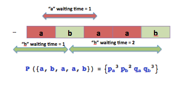
 Let's consider the following document composed by a sequence of two words: "a" and "b".

The Problem

• What is the probability function associated to a document Dk?

Given the following document:

The Probability of Dk is given by:

The below image should explain better what I meant:

Probability of Document Dk
q = 1-p

Probability Density Function 

-> From now, if not clearly specified I will refer to a document of two words (as above described).

Questions:

1. What is the analytical representation of the above function?
2. Is it the above function a probability function?

1. Analytical formulation

This is the funny part: I like combinatoric... the art of tally!

To solve the problem, I'm sure, there are several strategies, I used just the way that is more aligned to my mind setting: I put all the options on the table and I start to check to gather them together  according to some criteria :)

• The formulation of the "p" is a joke: the sum of the exponents must be equal to the size of the vector.
• the formulation for the "q" requires some deeper thinking.

As you know, I don't like too much technicalities, so I spare you the theoretical aspects.
I think it's more worthwhile  to show how the solution comes!

Exponents:
Let's put the q_a and q_b  exponents properly sorted on a matrix:

The split over the anti-diagonal makes the calculus easier.

Coefficients:

 The same configuration of exponents can be related to different configurations of the words in the document:

The different configurations (20) of two words in a document having length = 8. 

 Let's put the the occurrences of the different configurations of words for the same exponents configuration in a matrix:

# occurrences of the different configurations of words for the same exponents configuration.

Do you see the similarities respect the two halves of the matrix?

Is it easier now find the "low" to build the above matrix?

... If you don't like play around with combinatorics, you can ask help to  The On-Line Encyclopedia of Integer Sequences®!

Ok, ok you are too lazy...: the solution is Binomial[k+i,k].

The Analytical formula

The above matrixes suggest that the analytical formula is composed by two main addends: one for the orange side and another one for the green side.
For a document of two words the Probability Density Function is the following:

PDF for a document composed by two words.
qa = 1-pa = pb; pa+pb = 1.

I don't want enter in theoretical details to proof that the above formula is probability function (after all this is a blog by practical means!).
The only point I want to remark is that the convergence to a PDF is guaranteed for a length of document that tends to Infinity.
The above formula can be further reduced and simplified (in the easy case of 2 words) if you consider the following conditions:

qa = 1-pa = pb => qb=pa (pa+pb = 1).

Basically in the above case the PDF is function of 1 variable.

PDF and CDF for a document of 2 words.

In the CDF, we sum the probability contribute of all documents composed by two words having length =1, 2, ..., Infinity.
As you can see, the contribute of documents having length >50 is negligible for whatever value of pa.

These kind of distributions based on geometric variables are often used in maintenance and reliability problems, so I encourage you to have some reading on that!


Next Steps
In the next posts I'm going to explain

• some properties of the function
• its extension to multiple variables  
• entropy
• practical applications 

Last Consideration
I did the above exercise just for fun, with out any pretension to have discovered something new and or original: if you have some paper/book/reference about identical or similar work, please don't hesitate to contact me!

Don't rush, stay tuned
cristian

Image objects recognition: a basic approach

To complete the brief dissertation on the most popular problems of the image analysis science, I did a couple of experiments on a very intriguing topic: the identification of specific objects within an image.
I didn't use "state of art" algorithms (...my knowledge on the field is not deep and I wont use techniques that I don't fully understand!).
The target of this experiment isn't to show the best way, but just to show the rudiments of the matter.

Objective
Given an image called target image, and given another image called feature, the objective is to identify the features within the target image.

Technique 
I decided to play with a technique that I studied on signal processing course at University: the matrix correlation.

The matrix correlation is typically used to detect similarities between two 2D signals, which are often saved in matrices. 

The magnitude of the correlation shows how similar the signals are. If the correlation is large, the two signals are considered to be very similar. Alternatively, if correlation is zero, the two signals are considered to be independent. Analytical definition and explanation are available in all books of signal processing.

Experiment: Ball detection

In the first example I will try to detect the balls in the target image:

On the left the target image. On the right the feature (the ball!) to be identified in the image.

To solve the problem, I tried to apply the algorithm directly to the original images, but the results were terrible, so I applied some image manipulation technique in order to make more digestible the input to the main algorithm: I never be tired to say that preprocessing is crucial to solve a problem!

The algorithms used here are: edge detection and binarization. So I feed the correlation algorithm with the following input:

The input used to feed the correlation algorithm obtained with Binarization and eEge Detection techniques.

Results

Finally we can show the output: we can check if the algorithm identified correctly in the target image the balls!

To highlight the results I played around with colors and image merging :)

Results: balls identified in the image 

 As you can see the results are not so bad, and playing around with a preprocessing parameters I'm sure it's possible to improve the accuracy.

Experiment: Painting Recognition

I Applied the same technique to identify the paintings hung on a wall:

Target image: paintings hung on a wall

Results:

The techniques used are same of the above experiment, so let's go directly to the results:

Paintings detected

Considerations

The technique is quite rough and the accuracy depends on 

• Preprocessing technique applied 
• Measure used to compute the correlation (in both experiment I used cosine distance)

The algorithm per se seems to be not so general purpose to be used for such objective, but it's a good  starting point to approach the problem. Maybe if the feature to be detected is always the same (for instance as in face recognition), the accuracy is acceptable.

Stay Tuned

Cristian

Image comparison: SURF algorithm

In the former post I showed a naif approach that can be easily implemented and that works quite well under the condition that the image is not subjected to distortions.
I decided to deepen a bit the topic just for the sake of the curiosity ( curiosity and imagination are the skills that I most appreciate at work!).

SURF stands for "Speeded Up Robust Features" and it has been published by Herbert Bay, Andreas Ess, Tinne Tuytelaars, Luc Van Gool in 2008. The original paper is available here.

I strongly recommend to read the paper: it's self contained and it's very clear to be read also by neophyte  as I.
As usual I go straight to the experiments and to discuss the results.

Experiment
I considered again the same data set of the last post, and I tried to compare all the possible combinations  of pairs of images  to check the accuracy of the algorithm.

The first step of the algorithm is to determine the key features of an image.

key features detection

Once the features have been detected it's possible to use them for the comparison through euclidean measures or similar.

In the below image I plotted the common points and their position between two images:

Common points found between two images. In yellow I depicted them and their position.

If you zoom a bit the image you will notice that the common points found are thousands. To find them the algorithm took around four minutes.

In a productive environment this amount of time could be not acceptable. 

To improve the situation and reduce the computational time, I processed the image with binarization filters; after this preprocessing the time has been reduced from 4 minutes to 25 seconds.

Results

In the below matrix I listed all the comparison done to check the accuracy.

The correct pairs lay on the principal diagonal of the matrix.

In red have been listed the correct pairs

To show graphically the results I plotted over the matrix the number of common points found for each pair. The colors chosen highlight that number. 

Conclusions

As you can see for all the pairs on the principal diagonal the algorithm detected the highest number of common points.

In the next post I will show how to use this algorithm to identify logos in a document.

Stay tuned

Cristian

Image comparison for dummies: an easy and fast approach

Since I started to blog, I presented different methods, techniques and tricks to solve problems related to Data mining, and text mining (... I'm still puzzled about the difference between text mining and text analytics). 

Today I would like to present a different approach to solve a common problem in the text analytics area: the document comparison problem.

The problem
Usually if you want to compare two documents in order to check if they are pretty much the same you can apply some easy tricks in order to check frequency and position of the words.
Sometime the documents  require an OCR processing in order to get the "text rendition" for the documents, and such process usually is a very expensive in term of computational time (often it takes more than 10 seconds per page): what if you have to perform many comparison checks and you are short in time?
...In that case I suggest to consider the documents as images!

Image processing approach
This branch of the computer science evolved quite fast in the last decade and it achieves a level of complexity extremely high.
I'm not an expert at all, and many libraries (often free as opencv) are available and they offer several functionalities: image comparison, image recognition and so on.
Unfortunately I'm stubborn and curious and I like try to do experiments :).

So I decided to implement a very easy algorithm able to compare with high accuracy documents very similar.

Algorithm:
1. Resize the image (in order to have images having the same number of pixels)
2. Binarize the image
3. compute the histogram distribution
4. perform the comparison considering the Kullback distance between the two empirical distributions got from the histograms.

Considerations:

•  such algorithm is not robust to linear transformation/distortions of the image (but this is not case when you compare documents...).
• it's very fast respect the solutions that require OCR processing.
• it could be easily optimized considering sub-block of the images (and give higher weights to blocks in the middle of the image).
• through some assumptions based on eigenvectors it could be helpful also in case of image linear transformations.

Experiment

I selected 10 random images (pictures, medical analysis, text, screenshot):

Original sample set 

   

For each document, after some image adjust filter, I computed the histograms:

Histograms for the above images

I introduced some noise in each of the documents and I computed again the histograms:

Noised sample set.

Histograms for the noised images

As you can see, despite the noise introduced is quite big, the characteristic histogram seems to preserve quite well the shape.

Results:

I compared each possible possible combination of the pairs composed by original image and noised image and I ranked the result of the comparison.

...The test has been passed with an accuracy of 100%.

I have to say that the images are quite heterogeneous among each other, but further tests (I'll publish them in one of the next posts) highlighted that the method is quite robust (with all the limitations explained above).

Here is some of the best matching found:

Some of the best matching found

...I have to say that the image processing is a very fascinating  science!
Stay tuned
cristian