Image objects recognition: a basic approach

To complete the brief dissertation on the most popular problems of the image analysis science, I did a couple of experiments on a very intriguing topic: the identification of specific objects within an image.
I didn't use "state of art" algorithms (...my knowledge on the field is not deep and I wont use techniques that I don't fully understand!).
The target of this experiment isn't to show the best way, but just to show the rudiments of the matter.

Objective
Given an image called target image, and given another image called feature, the objective is to identify the features within the target image.

Technique 
I decided to play with a technique that I studied on signal processing course at University: the matrix correlation.

The matrix correlation is typically used to detect similarities between two 2D signals, which are often saved in matrices. 

The magnitude of the correlation shows how similar the signals are. If the correlation is large, the two signals are considered to be very similar. Alternatively, if correlation is zero, the two signals are considered to be independent. Analytical definition and explanation are available in all books of signal processing.

Experiment: Ball detection

In the first example I will try to detect the balls in the target image:

On the left the target image. On the right the feature (the ball!) to be identified in the image.

To solve the problem, I tried to apply the algorithm directly to the original images, but the results were terrible, so I applied some image manipulation technique in order to make more digestible the input to the main algorithm: I never be tired to say that preprocessing is crucial to solve a problem!

The algorithms used here are: edge detection and binarization. So I feed the correlation algorithm with the following input:

The input used to feed the correlation algorithm obtained with Binarization and eEge Detection techniques.

Results

Finally we can show the output: we can check if the algorithm identified correctly in the target image the balls!

To highlight the results I played around with colors and image merging :)

Results: balls identified in the image 

 As you can see the results are not so bad, and playing around with a preprocessing parameters I'm sure it's possible to improve the accuracy.

Experiment: Painting Recognition

I Applied the same technique to identify the paintings hung on a wall:

Target image: paintings hung on a wall

Results:

The techniques used are same of the above experiment, so let's go directly to the results:

Paintings detected

Considerations

The technique is quite rough and the accuracy depends on 

• Preprocessing technique applied 
• Measure used to compute the correlation (in both experiment I used cosine distance)

The algorithm per se seems to be not so general purpose to be used for such objective, but it's a good  starting point to approach the problem. Maybe if the feature to be detected is always the same (for instance as in face recognition), the accuracy is acceptable.

Stay Tuned

Cristian

Image comparison: SURF algorithm

In the former post I showed a naif approach that can be easily implemented and that works quite well under the condition that the image is not subjected to distortions.
I decided to deepen a bit the topic just for the sake of the curiosity ( curiosity and imagination are the skills that I most appreciate at work!).

SURF stands for "Speeded Up Robust Features" and it has been published by Herbert Bay, Andreas Ess, Tinne Tuytelaars, Luc Van Gool in 2008. The original paper is available here.

I strongly recommend to read the paper: it's self contained and it's very clear to be read also by neophyte  as I.
As usual I go straight to the experiments and to discuss the results.

Experiment
I considered again the same data set of the last post, and I tried to compare all the possible combinations  of pairs of images  to check the accuracy of the algorithm.

The first step of the algorithm is to determine the key features of an image.

key features detection

Once the features have been detected it's possible to use them for the comparison through euclidean measures or similar.

In the below image I plotted the common points and their position between two images:

Common points found between two images. In yellow I depicted them and their position.

If you zoom a bit the image you will notice that the common points found are thousands. To find them the algorithm took around four minutes.

In a productive environment this amount of time could be not acceptable. 

To improve the situation and reduce the computational time, I processed the image with binarization filters; after this preprocessing the time has been reduced from 4 minutes to 25 seconds.

Results

In the below matrix I listed all the comparison done to check the accuracy.

The correct pairs lay on the principal diagonal of the matrix.

In red have been listed the correct pairs

To show graphically the results I plotted over the matrix the number of common points found for each pair. The colors chosen highlight that number. 

Conclusions

As you can see for all the pairs on the principal diagonal the algorithm detected the highest number of common points.

In the next post I will show how to use this algorithm to identify logos in a document.

Stay tuned

Cristian

Image comparison for dummies: an easy and fast approach

Since I started to blog, I presented different methods, techniques and tricks to solve problems related to Data mining, and text mining (... I'm still puzzled about the difference between text mining and text analytics). 

Today I would like to present a different approach to solve a common problem in the text analytics area: the document comparison problem.

The problem
Usually if you want to compare two documents in order to check if they are pretty much the same you can apply some easy tricks in order to check frequency and position of the words.
Sometime the documents  require an OCR processing in order to get the "text rendition" for the documents, and such process usually is a very expensive in term of computational time (often it takes more than 10 seconds per page): what if you have to perform many comparison checks and you are short in time?
...In that case I suggest to consider the documents as images!

Image processing approach
This branch of the computer science evolved quite fast in the last decade and it achieves a level of complexity extremely high.
I'm not an expert at all, and many libraries (often free as opencv) are available and they offer several functionalities: image comparison, image recognition and so on.
Unfortunately I'm stubborn and curious and I like try to do experiments :).

So I decided to implement a very easy algorithm able to compare with high accuracy documents very similar.

Algorithm:
1. Resize the image (in order to have images having the same number of pixels)
2. Binarize the image
3. compute the histogram distribution
4. perform the comparison considering the Kullback distance between the two empirical distributions got from the histograms.

Considerations:

•  such algorithm is not robust to linear transformation/distortions of the image (but this is not case when you compare documents...).
• it's very fast respect the solutions that require OCR processing.
• it could be easily optimized considering sub-block of the images (and give higher weights to blocks in the middle of the image).
• through some assumptions based on eigenvectors it could be helpful also in case of image linear transformations.

Experiment

I selected 10 random images (pictures, medical analysis, text, screenshot):

Original sample set 

   

For each document, after some image adjust filter, I computed the histograms:

Histograms for the above images

I introduced some noise in each of the documents and I computed again the histograms:

Noised sample set.

Histograms for the noised images

As you can see, despite the noise introduced is quite big, the characteristic histogram seems to preserve quite well the shape.

Results:

I compared each possible possible combination of the pairs composed by original image and noised image and I ranked the result of the comparison.

...The test has been passed with an accuracy of 100%.

I have to say that the images are quite heterogeneous among each other, but further tests (I'll publish them in one of the next posts) highlighted that the method is quite robust (with all the limitations explained above).

Here is some of the best matching found:

Some of the best matching found

...I have to say that the image processing is a very fascinating  science!
Stay tuned
cristian

Mind maps of #textanalytics - automatic generation

What I want to show you today is "snippet" of a project I'm working during my spare time.
The project has the aim to gather, provide and represent the knowledge in a different way.
For the time being I don't want to disclose too much info, but the main idea is to leverage my concept of the graph entropy to capture information in a document (or in a data set) to create a new kind of indexer.

One of the output of the algorithm is the generation of the mind map.

Experiment
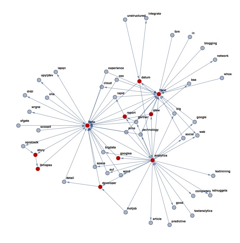
Through the API provided by Twitter I downloaded the last 200 tweets from the hashtag #textanalytics.
I processed the tweets and here is the results:

#textanalytics mind map

In red have been depicted the first 10 relevant words extracted through the graph entropy criteria.
It's interesting notice how the map shows intuitively the links among the words.
Of course the map can be enriched with more links or more relevant words: the choice depends on the user choice.
In the next posts I'll show you how the clustering techniques discussed in the former posts can be profitably used to create homogeneous group of words related each others.
what do you think?
Stay  tuned
cristian

Graph Clustering through "prominent vertexes": some clarification

I received many mails about the last post, and most of them asking explanations about the technique I developed.
I have to clarify that:

1. This method is just a consideration about the role played by some vertexes in a generic (directed) graph.
2. The results posted in the former graph can be a lot improved (I'm working on it among the several streams that I opened around the concept of entropy graph!).
3. the approach I'm going to explain in this post is not the same I used in the former because I prefer focus on the main idea respect the optimizations (but exential) aspects.

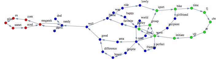
Let's consider the following graph:

Let's consider two nodes: "cbr" and "zx", then let's take all the paths that connect the two nodes:

All the possible paths between the node "cbr" and "zx"

We have now to consider the intersection (excluding the starting and ending points) among the all paths: 

such nodes are essential in order to reach the node "zx" from "cbr"because excluding just one of them, you cannot reach the ending point! 

The prominent nodes for the pair ("cbr","zx"): 

In the above procedure we found out the prominent nodes related to the pair "cbr", "zx".

Of course in order to determine the prominent nodes of the entire graph you have to consider all the pairs of nodes: that's the reason that justify the complexity >Binomial [n,2] of the procedure (n = order of the graph). The complexity doesn't consider the complexity to obtain the paths between the nodes!

The final result can be obtained taking the intersection of all "prominent nodes" for each pairs of nodes!

As you can imagine this is an expensive way to obtain the prominent nodes: I'll provide you an update about improvement on it.

Stay tuned 

cristian

Graph clustering: an approach based on "prominent vertexes"

I was doing some experiments on the entropy graph, and I noticed that under some conditions it is a good marker of special vertexes.
I'll try to explain the concept without formulas: that's really challenging because of my English :)
These vertexes play a special role that I decided (arbitrarily) to call "Prominent Vertexes": basically if you remove them, you introduce some disconnections on the graph; the remaining connected components are the clusters that induce the graph partitioning. To be more precise the connected components return just the N-1 clusters, the last cluster is obtained by the complement operation between the original graph and the N-1 clusters.

The intuitive explanation

• Consider all the possible paths between two nodes A and B in a graph
• Let's take for the above paths the intersection of them.
• The result is a set of nodes that are essential to connect the two nodes: these nodes are the prominent nodes for the vertexes A and B

The above schema can be applied (with some expedient) to all the Binomial[N,2] pairs of vertexes.

Some result

1st example

Let's consider the following graph and the respective "prominent vertexes":

In yellow have been depicted the prominent nodes for the graph

The clusters obtained considering the connected components are the following:

The 3 clusters obtained on the graph

As usual I compared my approach against another technique:  A. Clauset, "Finding Local Community Structure in Networks," Physical Review E, 72, 026132, 2005.

The 6 clusters obtained through the "Clauset" method.

Comment:

As you can see the proposed approach seems to be much less fragmented respect the Clauset method.

2nd example

Here is another example:

The 2 clusters obtained with the prominent vertexes method,

The 6 clusters obtained through the Clauset method.

Comment:

As in the former example the "prominent vertexes" method seems to behave better (even if the result is not optimal).

Considerations

PRO

• The method proposed seems to be a promising graph clustering algorithm.
• The method doesn't require parameters (e.g. number of clusters).
• The method doesn't fragment to much the nodes. 

CONS

• The complexity is (for the current implementation) quite high ~Binomial[Graph Order, 2].
• The method requires improvements and theoretical explanation.
• The method has lower accuracy when the vertexes degree is very small.

The code will be released as soon as the formalization of the Entropy Graph is completed.

Looking forward to receive your comments.

Stay tuned & Merry Christmas!

c. 

Document Clustering and Graph Clustering: graph entropy as linkage function

Let's continue our discussion about the applications of the graph entropy concept.
Today I'm going to show how we can re-use the same concept on the document clustering.
What I want to highlight is that through such methodology it's possible to:

1. extract from a document the relevant words (as discussed here);
2. clustering of the words of a document (as discussed here);
3. clustering set of documents;
4. clustering a graph and assign a ranking score to each cluster by homogeneity criteria;

The Experiment

For this experiment I chose a subset of the standard dataset called "the 20 Newsgroup dataset".

The documents of this data set are email selected from different newsgroups.

I selected some documents from the categories: Hockey, Motorcycle, Atheist and Electronics.

You can download here the documents used for this experiment.

The procedure 

• For each document build the respective graph (filtering by stopwords list, and stemming the words). 
• For each graph calculate the entropy graph value of each vertex (word).
• For each graph extract the first k relevant vertex (sorting by entropy graph value)
• Perform hierarchical clustering (in this case I used once again an approach based on Simulated annealing).

The results

Here you are the early results obtained through the clustering.

Each line depicts a cluster (the elements are the filename). The clusters have been sorted by homogeneity criteria assigned by the clustering algorithm. 

Considerations

The results are promising but not perfect. The accuracy achieved is

•  75.0% for first cluster 
• 62.5% for second cluster
• 50.0 % for the fifth cluster
• 37.5 % for the third and fourth cluster

The reasons of the bad aggregations are related to the class "atheist". Such class contains documents characterized by high variety: documents very short, text not strictly pertinent to the topic, topic quite general.

Moreover the clustering algorithm hasn't been optimized/customize for such problem.

Let's try to analyze the results under a different perspective:

Something more...

I mentioned before that such approach works over the concept of  entropy graph.

Here you are the graph representation of the words related to each cluster.

For each cluster I selected the first relevant 150 words.

In Red has been highlighted the first cluster

In dark Blue Has been Highlighted the second cluster

In Yellow has been depicted the third cluster

In Green has been depicted the fourth cluster.

In Brown has been depicted the fifth cluster.

Notes

Such representation of the clustering highlights that the linkage function used in this experiment depicts quite well the different areas of the graph.

• The Red cluster grouped together the right block of vertexes.
• The Brown cluster grouped the right side of the graph
• The Blue cluster focused on the core of the graph
• The yellow cluster grouped together the corona of the core of the graph
• The green cluster grouped together the corona of the peripheral of the graph.

The next steps

In the next post I'll try to refine the results, optimizing the clustering algorithm, and trying to use different kind of clustering algos.

Stay Tuned

cristian