Uncertainty coefficients for Features Reduction - comparison with LDA technique

We have already discussed about feature selection and features reduction, and all the techniques we explored were strictly related and applicable only in the text mining domain.

I would to show you one method very powerful, easy to implement and extremely general, because it is not related to the nature of the problem.

The method is known as coefficients of constraint (Coombs, Dawes and Tversky 1970) or uncertainty coefficient (Press & Flannery 1988) and it is based on the Mutual Information concept.


Mutual Information
As you know, the Mutual Information between two random variables X and Y I(X,Y) measures the uncertainty of X knowing Y, and it says how much the uncertainty (entropy) of X is reduced by Y.
This is more clear looking at the below formula:

I(X,Y)= H(X)-H(X|Y)

Where H is the Entropy functional.

As usual, I don't want enter in theoretical discussions, but I heartily recommend a deep read of the book Elements of Information Theory: In my opinion it's the best book in that field.

Let's now rethink the mutual information as a measure of "how much helpful is the feature X to classify documents having  label L":

I(L,X) = H(L)-H(L|X)

So, for each label and each features we can calculate the features ranking!

Of course you can consider the average of I(L_i,X) for each label L_i, or also more complex function over that. BTW you have to assign higher rank to the feature Xj that maximize all I(L_i,Xj).

Uncertainty coefficient

Consider a set of people's data labelled with two different labels, let's say blue and red, and let's assume that for this people we have a bunch of variables to describe them.

Moreover, let's assume that one of the variables is the social security number (SSN) or whatever univocal ID for each person.

Let me do some considerations:

1. If I use the SSN to discriminate the people belonging to the red set from the people belonging to blue set, I can achieve 100% of accuracy because the classifier will not find any overlapping between different people.
2. Using the SSN as predictor in a new data set never seen before by the classifier, the results will be catastrophic!
3. The entropy of such variable is extremely high, because it is almost a uniform distributed variable!

The key point is: the SSN variable could have a great  I value but it is dramatically useless to classification job.

To consider this fact in the "mutual information ranking", we can divide it by the entropy of the feature.

So features as SSN will receive lower rank even if it has an high I value.

This normalization is called uncertainty coefficient.

Comparative Experiment

Do you have enough about the Theory? I know that ... I did all my best to simplify it (maybe to much...).

I did some tests on the same data set used in this paper by Berkley University:

BleiNgJordan2003.pdf.

In this test the authors did a boolean experiment over REUTERS data set (actually it is very easy test) and they compared the accuracy obtained using all the words in the data set as features and the features extracted through a Latent Dirichlet Allocation method.

The data set contains 8000 docs and 15818 words. In the paper they claimed that they reduced the feature space by 99.6% and they used the entire data set to "extract" the features.

Under this condition they tested using no more than 20% of the data set as training set.

In the comparative test I focused on the second experiment mentioned: GRAIN vs NOT GRAIN.

Here you are the process I followed:

1. I choose as training set 20% of the docs.
2. from the above training set I extracted (after stemming and filtering process) all the words and I used them to build the boolean vectors.
3. I ranked the words through the uncertainty coefficient.
4. I extracted the first 60 features: that is only 0.38% of the original feature space
5. I trained an SVM with a gaussian kernel and very high value of C
6. I tested over the remaining 80% of the data set.

Before the results, let me show you some graph about the feature ranking.

Entropy of the first 3000 features.

The above graph shows the entropy of the first 3000 features sorted by TF-DF score.
As you can notice, the features having low score have low entropy: it happens because these features are present in really few documents so the distribution follows a Bernulli's distribution having "p" almost equal to 0: basically the uncertainty of the variable is very small.


Here you are the final ranking of the first 2500 features. 

Uncertainty coefficient for all features.

Results

The overall accuracy measured over the test set is equal to 96.89% and it has been depicted in the below graph (I used their original graph [figure 10.b] as base) as a red circle:

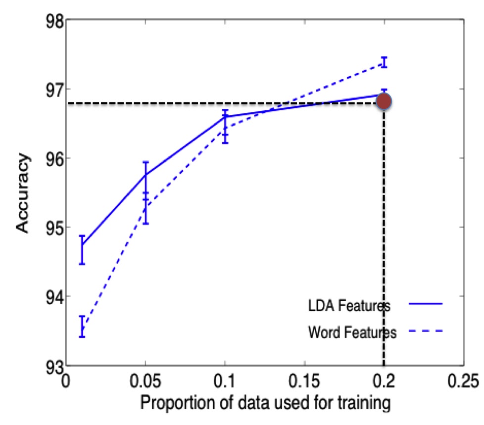
Accuracy comparison: the red circle represents the accuracy obtained training an SVM with the features extracted through the Uncertainty Coefficients.

I would like to remark that the features has been extracted using just the training set (20% of the data set),  while the experiments done by the authors of the mentioned paper used the entire data set.

Better results can be easily achieved using the conditioned entropies in an iterative algorithm where the mutual information is measured respect a local set of features (adding the features that maximize the M.I. of the current set of features).

Our  experiment shows clearly that the "Uncertainty Coefficients" criteria is a really good approach!

Soon, we will see how to use this criteria to build a clustering algorithm.  

As usual: stay tuned.

cristian

Earthquake prediction through sunspots part II: common Data mining mistakes!

While I was writing the last post I was wondering how long before my followers notice the mistakes I introduced in the experiments.
Let's start the treasure hunt!
1. Don't always trust your data: often they are not homogeneous.
In the post I put in relation the quakes in the range time between [~1800,1999] with the respective sunspots distribution.

A good data miner must always check his dataset! you should always ask to yourself whether the data have been produced in a congruent way.
Consider our example: the right question before further analysis should be: "had the quakes magnitude been measured with the same kind of technology along the time?"
I would assume that is dramatically false, but how can check if our data have been produced in a different way along the time?
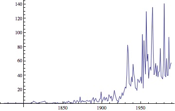
In this case I thought that in the past, the technology wasn't enough accurate to measure feeble quakes, so I gathered the quakes by year and by the smallest magnitude: as you can see, it is crystal clear that the data collected before 1965 have been registered in different way respect the next period.

The picture highlights that just major quakes (with magnitude > 6.5) have been registered before 1965.
This is the reason of the outward increasing of quakes!

... In the former post I left a clue in the caption of "quakes distribution" graph :)

In this case the best way to clean up the dataset is to filter just quakes having magnitude grater than 6.5.

Let me show you a different way to display the filtered data: "the bubble chart".

The size of the bubble is representative of the magnitude of the quakes 

The size of the bubble is representative of the number of the quakes

I love the bubble chart because it is really a nice way to plot 3D data in 2D!!

2. Sampling the data: are you sampling correctly your data?

In the former post I considered only the quakes registered in USA. 

Is it representative of the experiment we are doing?

The sunspots should have effects on the entire Earth's surface, so this phenomena should produce the same effects in every place.

...But as everybody knows: there are regions much more exposed to quakes respect other areas where the likelihood to have a quake is very low.

So the right way to put in relation the two phenomena is to consider the World distribution of the quakes.

3. Don't rely on the good results on Training Set.

This is maybe the worst joke I played in the post :) I showed you very good results obtained with the support regression model.

...Unfortunately I used the entire data set as training set, and I didn't check the model over a new data set!

This kind of mistake in the real scenario, often generates false expectation on your customer.

The trained model I proposed seemed very helpful to explain the data set, but as expected it is not able to predict well :(.

How can you avoid the overfitting problem? The solution of this problem is not so trivial, but in principle, I think that cross validations techniques are a safe way to mitigate such problem.

Here you are the new model:

The left graph shows the Training Set (in Blue the number of quakes per year, in Red the forecasting model).
The graph on the right side shows the behavior of the forecasting model over a temporal range never seen before by the system. The mean error is +/-17 quakes per year.

The Magnitude forecasting
(on the left the training set, on the right side the behavior of the forecasting model over the test set).
The mean error is around +/-1.5 degrees.

Considering the complexity of the problem I think that the regressor found works pretty good.

Just to have a better feeling of how the regressor is good, I smoothed the data through a median filter:

Moving Median Filtering applied to the Magnitude regressor.

Looking at the above graph, it seems that the regressor is able to follow the overall behavior.

As you can see such filtering returns a better understanding of the "goodness" of your models when the function is quite complex.

4. You found out a good regressor, so the phenomena has been explained: FALSE.

You could find whatever "link" between totally independent phenomena ... but this link is just a relation between input/output. nothing more, nothing less.

As you know this is not the place for theorems, but let me give you a sort of empirical rule:

"The dependency among variables is inverse proportional to the complexity of the regressor".

As usual stay tuned.

Cristian

Support Vector Regression (SVR): predict earthquakes through sunspots

In the last months we discussed a lot about text mining algorithms, I would like for a while focus on data mining aspects.
Today I would talk about one of the most intriguing topics related to data mining tasks: the regression  analysis.
As you know the regression analysis is an approach to modeling the relationship between a set of variables "y" and  explanatory variables "x" (called regressor).
The model I've chosen to talk about regression is strictly related to the SVM algorithm already presented in our classification problems: Support Vector Regression (SVR).


How does it work?
In SVR the basic idea is to map the data x into a high-dimensional feature space F via a nonlinear mapping  and to do linear regression in this space.


Why SVR?

• SVR is extremely robust even in input space having high dimension because the optimization doesn't depend on the dimension of input space.
• SVR depends only on a subset of the training data, because the cost function for building the model ignores any training data close to the model prediction.
• SVR over ordinary linear regression has the advantage  of using a large variety of loss functions to suit different noise models.
• SVR is more robust than linear regression for noise distributions close to uniform.

I don't want spend words about the theory, there are several tutorials on it downloadable from scholar google.

Applications

The regression models are widely used to infer a phenomena through several variables. Financial forecasting, risk management, clinical tests,  are just examples of areas where these techniques are applied.

Consider for instance earthquake events: imagine for an insurance company how can be relevant assign a risk score to define the right premium for such risk.

For this kind of market a predictor based on other variables already available or at least on variables easier to predict could represent a solid base to assess the right price for the premium and, the discovery of new predictors could represent a huge advantage respect competitors.

...Let's try to play with SVR:

Experiment: Earthquakes prediction using sunspots as regressor

Early warning: this is just a tutorial, so don't consider the results of this experiment as a real scientific work on earthquake prediction!

Data considered:

- series of earthquakes registered in USA since 1774 to 1989.

- series of sunspots registered since 1774 to 1989.

Let's plot the graph of the number of quakes registered per year and the related number of sunspot:

The two coplanar axis are respectively the "time line" and "# sunspots", the z axis represents the number of earthquake registered.    

As you can see the graph shows a significant increasing of the number of earthquakes registered when the number of sunspots are dramatically low and high.

What about the magnitude? 

The two coplanar axis are respectively the "time line" and "# sunspots", the z axis represents the highest magnitude of earthquakes registered. 

The above graph returns exactly the same information: to low number of sunspots or high number of sunspots corresponds to higher magnitude of earthquakes.

Support Vector Regression

I removed the time line axis; the below graph shows the number of earthquakes and the respective number of sunspots:

On X axis # sunspots, on Y axis # earthquakes.
(the point have been joined just for the sake of clarity)

I played a bit with Gaussian kernels, and here you are the results of the SVR regression:

In Red the original data, in Blue the predicted data. 

As you can see the model is extremely precise especially when the sunspots are greater than 50.

For low values of # sunspots the predictor tends to underestimate the number of earthquakes occurred.

Same considerations in prediction of magnitude:

We will see how to improve the accuracy.

Stay tuned!

cristian 

Appendix

Sunspot series:

Sunspots series

Earthquake series:

Earthquake series.
... The increasing of number of quakes is suspicious.  

The regressor found:

Features Extraction: Co-occurrences and Graph clustering

In the last two post we have discussed about co - occurrences analysis to extract features  in order to classify documents and extract "meta concepts" from the corpus.
We have also noticed that this approach doesn't return better than the traditional bag of words.
I would now explore some derivation of this approach, taking advantage of the graph theory.

In the following step I'm gonna to show you the alternative strategy applied to a corpus for the category "GRAIN" (referred always to our official data set REUTERS 21578).

Co - occurrences 
The first step is to extract the co occurrences as we already explained in the former posts.
The test has been performed considering just 100 documents, below the graph showing the score assigned to all (>5000) co occurrences extracted by the proc.

Sorted score assigned to the co occurrences extracted from the GRAIN category (100 docs).

Graph Reduction
In this step we build the graph of the co-occurrences of two words to obtain a representation of the links among the other co occurrences.
Here you are the graph obtained from this step:

The Graph of the co-occurrences linkage for the GRAIN category

 As you can see the graph is really huge and complex, how could we reduce its complexity without big information loss?
The Kcore algorithm could help in doing that. It gives groups of vertices that are connected to at least k others.
To build it you can remove repeatedly vertices of out-degree less than k.
Below the k core components from the original graph (the k chosen here is five).

k core components extracted from the original graph 

This reduction reduced the number of nodes from 5163 to 104.

The entities extracted

Form the k-core graph we could extract the shortest path for each combination of two vertexes.

And we can compare the paths obtained with the document in the corpus to select the paths really existing in the documents (this trick of course should be applied only on the training set!).

The procedure returned 526 entities.

Here you are the longest entities extracted:

1 rice farmer reach acre

2 department say last summer

3 contract trade  agricultural

4 month pct increase

5 summer grain harvest

6 board trade agricultural

7 record tonne previous

8 rice farmer reach

9 cash crop include

10 high rate national

11 pay crop loan

12 cotton payment reach

13 major farm group

14 future year ago

15 future trade area

16 total tonne intervention

17 offer  exporter issue

18 import tonne agricultural

19 bushel price  current

20 bushel corn producer

The graph clustering

Another interesting things we can do with such entities  is to isolate in the kcore graph the nodes that describe the entities and apply a clustering algorithm over the graph connections.

I decided to apply in this case as a clustering distance the "community modularity".

The clustering returns unstructured features.

Here you are the clustered graph and the unstructured features clustered:

The clustered k-core graph

The unstructured features clustered

As you can see last step tends to group together words semantically related:

Consider for example the second cluster, it contains almost all words related to period of time topic as "winter, year, month, ago", the fourth represents political aspects, the fifth describes quite precisely economic aspects.

The third cluster is gathering aspects strictly related with the main topic "grain", while the first one seems group words not related with the topic.

Of course it's not 100% accurate, and is still open the question how to use this clusters.

In the next post I'm gonna extend this experiment to other categories, and I would like to check if the entities extracted can be used to improve the accuracy of our classifier.

...Stay tuned

cristian

Document Classification: latent semantic vs bag of words. Who is the best?

We have seen few posts ago an approach to extract meta "concepts" from text based on latent semantic paradigm.
In this post we apply this approach to classify documents, and we do a comparison between this approach and the canonical bag of words.
The comparison test will be done through the ensemble method already showed in the last post.

Features
The idea is to build the features set considering constructs of co-occurrences instead of single words as usually done with bag of words.

• The prominent advantage of this approach is well rendered when the corpus contains structured features as for instance "bank account, invoice number" and so on. 
• The biggest disadvantage lays in the length of the feature set and consequently in the length of the vectors built to represent each document.

Let me clarify the last point: consider for instance a corpus of 100 words; in this case the dimension of each vectors will be less or equal to 100. Let's try now to consider the co-occurrences of these 100 words, and just to simplify the process, let's focus on the co-occurrences of two words (so we consider the closeness of two words), in this case the length of the vector is 100*100 =10000!!.

The image below represents the graph of the co-occurrences extracted considered the highest ranking (the ranking has been assigned in the way described in this post applied to the data set used to explain the ensemble method based on ADA boost M1).

The most important features extracted through the LSA method.

Vectors
To build the vectors I used the first 15000  structured features extracted by the latent semantic method and I considered just features composed by 2 words (co-occurrences).
To mitigate the complexity to crunch vectors with dimension so high, I built the training and test set using sparse matrixes of boolean values.
The advantage of the sparse matrix working with SVM is related to the small memory consumption required to select the support vectors.
Someone could argue that inner product of sparse array requires additional effort in the kernel evaluation, but if the vectors contain only boolean values, this extra complexity is negligible.

Comparison
To perform a comparison test, I used the same sets and the same strategies of learning.
In both scenarios, I trained the system through the ensemble techniques described in the last post (based on the boos method of ADA boost M1).

Results:
Before to discuss the results let me show the confusion matrixes.

Confusion Matrix for LSA based classifier.
(How to read it?...look at the former post)

Confusion Matrix for "Bag of Words" based classifier.
(How to read it?...look at the former post)

In blue it has been represented the results for LSA based approach.
In red it has been represented the results for Bag of Words approach.

As you can see, even if the results obtained with the LSA classifier are not so bad, the traditional approach based on bag of words (in this experiment extracted through TD-DF) returns better results.

Why?

The training set used generated around 8.000 features (single words) and the vectors have been built using 500 features (6.25% of the total). 

The size of the features having relevant ranking in the LSA approach is around 15000, and to ensure the same conditions of the test I trained the system choosing again 500 features (3.33% of the total).

Basically the useful information to classify the docs in LSA approach is spread over a bigger feature set.

Conclusion
As we have already seen in the past, doesn't exist a technique that perform better than other approaches with every data set. With this data set (a sub set of the Reuters 21578) the LSA requires more physical resources and returns worse results.

If we scratch the surface of the results, we can observe that it detects different aspects of the corpus to classify the docs: for instance it performs better with "GRAIN" category. So I wonder if we can take advantage of this aspect to ensemble this approach with the bag of words to improve further the accuracy (as suggested by a follower of this blog) !
...We will see the results of this conjecture the next post.
As usual: Stay Tuned!!
Cristian

Document Classification: how to boost your classifier

Time ago, we discussed about ADAboost as a meta algorithm useful to improve the accuracy of a weak classifier and I showed a sample on a boolean classification problem.
Frund and Schapire in this excellent paper proposed a version of this algorithm adapted to work with "multi labels" classifiers.

The two variants proposed in such paper are based on the trick to assign a weight to each sample of the training set in according with the error committed by the classifier, so it forces the classifier to be focused on the hard instances of the problem.
The improved classifier is finally obtained as a weighted combination of each version of the weak algorithm improved at each iteration.

Adaption of AdaBoost.M1 to a classifier SVM based.

ADaBoost.M1 tries to improve step by step the accuracy of the classifier analyzing its behavior on training set. (Of course you cannot try to improve the classifier working with the test set!!).
Here lays the problem, because if we choose as "weak algorithm" an SVM, we know that almost always it returns excellent accuracy on the training set with results closed to 100% (in term of true positive).
In this scenario, try to improve the accuracy of classifier assigning different weights to the training set doesn't work!

The idea of AdaBoost.M1 is still valid also with SVM classifiers, but I noticed that instead of to improve step by step the single SVM classifier,  we can train different SVM classifiers (with different parameters) and assign the score to each classifier based on the error committed on a part of the training set not used to train the SVM.
Let me explain better the procedure:

1. Split the training set in two different sets: training set (80% of the volume of the original training set), boosting set (20% of the volume of the original training set).
2. train k SVM classifiers with different parameters.
3. test the above SVM on the boosting set and calculate the beta score as done in the original implementation of ADAboost.M1.
4. The final answer of the boosted classifier is obtained as proposed by the original implementation of the Adaboost.M1

As you can notice, the method basically assigns to the k classifiers a "trustability score".


Real Case
Let's see what happens with our REUTERS-2158 data set:
I tried to classify the documents belonging to the categories: "GRAIN","CRUDE", "TRADE","OIL".
I trained four different SVM. Here you are what are the results of each classifier:

The Confusion Matrix for the Classifier I.The principal diagonal represents the True Positive.
In The circle the worst result for this classifier.

The Confusion Matrix for the Classifier II.The principal diagonal represents the True Positive.
In The circle the worst result for this classifier. 

The Confusion Matrix for the Classifier III.The principal diagonal represents the True Positive.
In The circle the worst result for this classifier. 

The Confusion Matrix for the Classifier IV.The principal diagonal represents the True Positive.
In The circle the worst result for this classifier. 

And after the application of the meta algorithm, here you are the confusion matrix for the improved classifier:

The Confusion Matrix for the Boosted classifier

As you can see the boosting provides us really good results! 

Here the same results showed in terms of precision and recall:

 

The Precision/Recall chart for the four weak classifiers.
(The ring shows the worst case for each classifier)

And here you are the Precision/Recall for the boosted classifier:

As usual Stay Tuned

Cristian

Extract meta concepts through co-occurrences analysis and graph theory.

During The Christmas period I had finally the chance to read some papers about probabilistic latent semantic and its applications in auto classification and indexing.

The main concept behind “latent semantic” lays on the assumption that words that occurs close in the text are related to the same semantic construct.

Based on this principle the LSA (and partially also the PLSA ) builds a matrix to keep track of the co-occurrences of the words in text, and it assign a score to these co-occurrences considering the distribution in the corpus as well.

Often TF-IDF score is used to rank the words.

Anyway, I was wondering if this techniques could be useful also to extract key concepts from the text.

Basically I thought: “in LSA we consider some statistics over the co-occurrences, so: why not consider the link among the co-occurrences as well?”.

So what I did is the following (be aware that is not the formal implementation of LSA!):

1. Filter and take the base form of the words as usual.
2. Build the multidimensional sparse matrix of the co-occurrences;
3. I calculated for each instance the frequency to find it in the corpus;
4. I calculated for each instance the frequency to find it in the doc;
5. I weighted such TF-IDF considering also the distance among the co-occurrences.

In this way we are able to rank all co-occurrences and set a threshold to discard items having low rank.

In the last step I built a graph where I linked the co-occurrences.

As you can see in the following examples, the graphs are initially pretty complex, and to refine the results, I applied filter based on the number of connected components in the graph.

The below examples are representing the concepts extracted by the first three chapters of the books “The Media in the Network Society, author: Gustavo Cardoso” Available at http://ebooksgo.org/computer/networksecurity.pdf

Meta - concepts (unfiltered) extracted from "Introduction" chapter.

Meta - concepts (unfiltered) extracted from "Introduction" chapter.

The arrows, help to identify correct direction to read the "meta concepts". Of course is still required a bit of efforts to identify the underlying semantic but after a quick reading of the original source is easy convince oneself that this representation fits pretty good with the content.

Below the outcomes for the first chapter:

Unfiltered meta concepts for the first chapter

Filtered meta concepts for the first chapter

And, here you are the the second chapter:

Unfiltered meta concepts for the second chapter

Filtered meta concepts for the second chapter

I'm sure that there is room to big improvements of this rough method, for instance assigning the ranks of the co-occurrencies with more sophisticated ways respect the usual TF-IDF (like using centrality based measures, or considering cosine distances).

Are these constructs also useful to classify text?

…we will see the answer in the next post J.

Stay tuned

cristian